How to Solve Complex Regression Modelling Assignments in Statistics

Your first step is to decode the data structure. Assignments like these usually present you with a multivariable dataset — typically involving both quantitative and qualitative variables. For example, a hospital-based dataset may contain:

• Continuous variables: Average age of patients, number of beds, length of stay, infection risk percentage, nurse count.
• Categorical variables: Medical school affiliation (yes/no), geographic region (NE, NC, S, W).

Before running any models, explore these variables:

• Use str() in R to check variable types.
• Manually convert any incorrectly classified variables using factor() for categorical ones.
• Use summary() and table() for univariate summaries.

Key takeaway: Proper classification of variables lays the foundation for accurate Modelling.

2. Initial Data Exploration: Visualization and Descriptive Statistics

Descriptive statistics and visual diagnostics should always precede Modelling. Begin with:

• Boxplots to examine how a continuous outcome (e.g., length of hospital stay) varies across categorical groups.
• Scatterplots for exploring pairwise relationships among continuous predictors.
• Correlation matrices to check collinearity risks.

This step gives insight into potential relationships, outliers, and group effects. For example, if average age and infection risk both seem related to length of stay in preliminary scatterplots, they become prime candidates for regression predictors.

Example Equation (only 1 here, as per guideline):

LengthStayi = β0 + β1⋅Agei + β2⋅InfectionRiski + ϵi

3. Fitting a First-Order Regression Model

In a typical assignment, you're asked to build a first-order (linear) regression model involving both continuous and categorical predictors. Here's how you do it:

• Use lm() in R to fit the model.
• For categorical variables, R automatically uses dummy coding if they are factor objects.
• Examine the output from summary(model).

At this stage, your interpretation should focus on:

• Significance: Which variables are statistically significant?
• Signs of coefficients: Do they match your expectations (e.g., higher infection risk leading to longer stays)?
• Magnitude: Are changes in the outcome practically meaningful?

Important Tip: Always interpret coefficients within the context of other variables being held constant.

4. Model Comparison and Variable Significance

Most regression-based assignments require you to test if a subset of variables (often categorical) can be dropped without harming model performance.

Steps:

• Use the ANOVA function anova(model1, model2) for nested model comparisons.
• Evaluate F-statistics and p-values.
• Use adjusted R² as a secondary model performance measure.

Removing insignificant variables often leads to a more parsimonious model — but statistical tests must support your decision.

Model selection criteria:

• Higher Adjusted R²
• Lower SSE (Sum of Squares Error)
• Favorable AIC/BIC values

5. Interaction Effects: When Variables Work Together

Many assignments test your ability to identify and evaluate interaction terms. For example, interaction between age and infection risk might reveal whether older patients with high risk stay significantly longer in hospitals.

To test:

• Add interaction terms like Age:InfectionRisk in the model.
• Interpret the interaction coefficient.
• Visualize with ggplot2 using geom_smooth(method="lm") with color=Region or similar groupings.

Interpretation Strategy: If the interaction term is significant and the coefficient large, the effect of one predictor varies depending on the level of the other — a non-trivial insight in health-related studies.

6. Prediction and Interval Estimation

Once you finalize a model, assignments often ask for interval estimates:

• Confidence Intervals for mean response
• Prediction Intervals for individual outcomes

Use predict() in R:

predict(model, newdata = hospital_profile, interval = "prediction", level = 0.90)

Be clear whether the interval relates to an individual hospital or to the average for a group of hospitals. The intervals help interpret uncertainty and apply your model practically.

7. Advanced Model Diagnostics and Variable Reconsideration

Later parts of the assignment usually reintroduce additional predictors (e.g., daily census, facility index). Here's the approach:

• Fit the extended model.
• Examine any drastic coefficient sign changes or significance shifts.
• Use Variance Inflation Factors (VIF) to check for multicollinearity.
• Justify inclusion or exclusion based on theory and model performance.

When signs flip or p-values jump: That’s a red flag. Investigate whether:

• New variables are collinear with existing ones.
• The dataset lacks sufficient variation.
• The underlying causal assumptions need refinement.

8. Group Differences and Dummy Variable Interpretation

When comparing group effects — say, between hospitals in the NC vs. Southern regions — you must interpret categorical coefficients correctly.

In R:

• A baseline category is automatically chosen.
• Coefficients for other categories represent differences from that baseline.

To compare two non-baseline groups, compute:

(β^NC − β^S) ± CI width

And use contrasts via contrasts() or releveling the factor.

Assignments may require formal hypothesis testing for such differences. You can use:

• linearHypothesis() from the car package
• or manual calculations based on coefficient estimates and standard errors.

9. Multivariate Confidence Intervals (Bonferroni Approach)

Bonferroni joint confidence intervals are often requested for all quantitative variable coefficients. Why Bonferroni?

It adjusts for multiple comparisons and protects against Type I error inflation.

To construct:

• Use confint() or manually with:

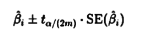
where m = number of comparisons.

This shows you're aware of the multiple inference context — crucial in policy-oriented datasets like those in healthcare.

10. Visualizing Model Fits by Groups

Assignments that ask whether an effect (e.g., infection risk) differs across regions test your understanding of interaction plots and stratified regression lines.

Steps:

• Use ggplot2 to color lines by geographic region.
• Add interaction terms like InfectionRisk:Region in the model.
• Plot and interpret.

If interaction terms are significant and slopes differ visibly across regions, you can conclude the effect of infection risk is region-dependent.

Conclusion

These assignments aren’t just about executing R code — they’re about statistical storytelling. Every model choice, interaction term, or exclusion has to be explained, backed by theory, and supported with evidence from the data.

Here’s a checklist to wrap up your submission:

• All variables correctly typed (factor vs. numeric)
• Exploratory plots included and interpreted
• Regressions built incrementally with justification
• Model comparison tests conducted and explained
• Confidence/prediction intervals computed appropriately
• Visualizations clearly annotated
• Hypotheses tested formally and interpreted
• Report structured logically with clear headings
• Appendix includes well-commented R code

Remember: Regression Modelling is as much about communication as it is about computation.