Statistical Analyses Homework Help

One-Way ANOVA

A. One way Anova will be used a statistical test that compares the difference in the group means of a categorical dependent variable against the continuous independent variable. In this case race is the categorical independent variable with 3 levels (white, African Americans and Others), while SAT_R_pre is the continuous independent variable.

ANOVA
Stanford Achievement Test NCE scores in Reading Before
	Sum of Squares	df	Mean Square	F	Sig.
Between Groups	2341.061	2	1170.530	3.426	.036
Within Groups	42360.337	124	341.616
Total	44701.397	126

Interpretations: “A one-way between subjects ANOVA was conducted to compare the difference in the Pre-SAT reading scores among different races. There was a statistical significant difference in the Pre-SAT reading scores of the three different race with (F=3.426, p=0.036).

C. t tests - Means: Difference between two independent means (two groups)

Analysis: A priori: Compute required sample size

Input: Tail(s) = Two

Effect size d = 0.5

α err prob = 0.05

Power (1-β err prob) = 0.80

Allocation ratio N2/N1 = 1

Output: Noncentrality parameter δ = 2.8284271

Critical t = 1.9789706

Df = 126

Sample size group 1 = 64

Sample size group 2 = 64

Total sample size = 128

Actual power = 0.8014596

Using G-power analysis the required sample size is 64 for group 1 and 64 for group 2 which will amount to 128 total sample size.

Two-Way ANOVA

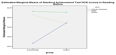
A. Two- Way ANOVA is the appropriate statistical level to use. The two-way ANOVA is used to estimate how the mean of a quantitative variable changes according to the levels of two categorical variables. In this question both race and group are the categorical variables while the Pre-SAT reading scores is the dependent variable.

a. R Squared = .080 (Adjusted R Squared = .042)

Tests of Between-Subjects Effects
Dependent Variable: Stanford Achievement Test NCE scores in Reading Before
Source	Type III Sum of Squares	df	Mean Square	F	Sig.
Corrected Model	3596.055^a	5	719.211	2.117	.068
Intercept	333707.428	1	333707.428	982.320	.000
group	84.123	1	84.123	.248	.620
race	2976.851	2	1488.425	4.381	.015
group * race	1064.266	2	532.133	1.566	.213
Error	41105.342	121	339.714
Total	486021.730	127
Corrected Total	44701.397	126

Interpretations: A two way analysis of variance was conducted to examine if there is a difference in Pre-SAT reading scores according to group and race. We can see from the table above that there was no statistically significant difference in mean of Pre-SAT reading scores for the two groups (F=0.248, p = .620), but there were statistically significant differences between the three race (F=4.381, p < .0005).

C. Plot of cell means

D. Post hoc test for race against Pre-SAT reading scores.

Multiple Comparisons
Dependent Variable: Stanford Achievement Test NCE scores in Reading Before Tukey HSD
(I) race	(J) race	Mean Difference (I-J)	Std. Error	Sig.	95% Confidence Interval
(I) race	(J) race	Mean Difference (I-J)	Std. Error	Sig.	Lower Bound	Upper Bound
African American	White	-9.505^*	3.6212	.026	-18.098	-.913
African American	Others	-5.740	4.9706	.482	-17.535	6.054
White	African American	9.505^*	3.6212	.026	.913	18.098
White	Others	3.765	4.7305	.706	-7.460	14.990
Others	African American	5.740	4.9706	.482	-6.054	17.535
Others	White	-3.765	4.7305	.706	-14.990	7.460

Interpretations: From the table above we can see that there is a statistical significance between Pre-SAT scores of White and African Americans race with (p>0.005) while there is no significance pairs of relationship among other race.

E. F tests - ANOVA: Fixed effects, special, main effects and interactions

Analysis: A priori: Compute required sample size

Input: Effect size f = 0.8

α err prob = 0.01

Power (1-β err prob) = 0.8

Numerator df = 2

Number of groups = 2

Output: Noncentrality parameter λ = 17.2800000

Critical F = 5.5679971

Denominator df = 25

Total sample size = 27

Actual power = 0.8141890

From the G-power test above the required sample size is 27.

Correlation Analysis

A. Correlation Analysis will be used. The correlation analysis is a statistical techniques that is used to measure the relationship that exists between continuous variables.

Correlations
		Stanford Achievement Test NCE scores in Reading After	Stanford Achievement Test NCE scores in Language After	Stanford Achievement Test NCE scores in Math After
Stanford Achievement Test NCE scores in Reading After	Pearson Correlation	1	.737^**	.789^**
	Sig. (2-tailed)		.000	.000
	N	148	148	148
Stanford Achievement Test NCE scores in Language After	Pearson Correlation	.737^**	1	.738^**
	Sig. (2-tailed)	.000		.000
	N	148	148	148
Stanford Achievement Test NCE scores in Math After	Pearson Correlation	.789^**	.738^**	1
	Sig. (2-tailed)	.000	.000
	N	148	148	148

**. Correlation is significant at the 0.01 level (2-tailed).

Interpretations: From the table above, we found a strong significant relationship between Stanford Achievement Test NCE scores in Reading After and Stanford Achievement Test NCE scores in Language After with (r=0.737, p<0.05). Similarly, there is a strong significant positive relationship between Stanford Achievement Test NCE scores in Reading After and Stanford Achievement Test NCE scores in Math After with (r=0.789, p>0.05). Lastly, there is strong significant relationship between Stanford Achievement Test NCE scores in language After and Stanford Achievement Test NCE scores in Math After with (r=0.738, p<0.05).

C. t tests - Correlation: Point biserial model

Analysis: A priori: Compute required sample size

Input: Tail(s) = Two

Effect size |ρ| = 0.8

α err prob = 0.05

Power (1-β err prob) = 0.8

Output: Noncentrality parameter δ = 3.5276684

Critical t = 2.5705818

Df = 5

Total sample size = 7

Actual power = 0.8029379

From the G-power test above, the total sample size is 7.

Reliable Statistical Analyses Homework Help

One-Way ANOVA

Two-Way ANOVA