Using SAS to check motor sales
Here we will use SAS to check motor sale trends for a three-month period. We will use a regression model to interpret the results.
Your organization has collected sales data on its small engine product sold and distributed from 6 different locations: Kansas City, Chicago, Houston, Oklahoma City, Omaha, and Little Rock. The organization wants to predict motor sales for the next three months for each location. Your task is to conduct predictive analytics statistical tests on a sample data set named “MotorSales.csv” (Please find the file attached). You are expected to perform the appropriate regression statistics tests and prepare the appropriate tables, charts, and graphs needed to predict future sales. You must provide an alternate and null hypothesis. In a paper document, Submit the following items for this assignment:
- Submit Screenshots of the results for each statistical test including any charts, graphs, and tables. Include the date and time for each screenshot capture.
- Submit the Alternate and null hypotheses for each business question.
- Submit Projections for 3 months of future sales for each location.
- What business insights can the company gain from the results of this test? Your paper must be at least five pages minimum in length (including the screenshots images).
In support of your response, cite and integrate at least two scholarly sources. Please submit all of the steps, as far as the SAS programming codes that were used, and done in SAS.
Solution:
Forecasting is very important for any business to survive in the competitive world. A reliable forecast makes strategic planning, which is essential for a company operating in a market environment, easy (Hulsmann et al., 2012). The purpose of a sales forecast is to predict future sales and this will help the management to plan production and necessary materials needed for production (Sharma, 2012). The purpose of this work is to forecast the next three months' sales of small engine products for six locations. The locations are Kansas City, Chicago, Houston, Oklahoma City, Omaha, and Little Rock. The regression model was used to achieve this aim. The independent variables used are first lag of sales, month dummies location dummies, and trend.
The null and alternative hypothesis is given as
H01: previous period sales has no significant effect on sales
H11: previous period sales has significant effect on sales
H02: Auto Sales does not significantly differs by location and time
H12: Auto Sales differs significantly by location and time
H03: Auto sales has no significant trend
H13: Autosales has no significant trend
The first stage of the analysis is to read the dataand convert the data from wide format to long format. This was done in SAS and the screenshot for the data importing and converting stage is presented in fig 1. The dataset contains 24 observations for each of the location.
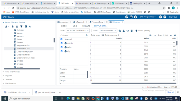
Fig 1: Data Import
Next, we graph the sales variable for each location. The plot is presented in figure 2. The plot shows that auto sales for Chicago follow an upward trend while sales for OKcity follow a significant downward trend. The auto sales for Houston follow an upward trend initially followed by a downward trend after around ten months.
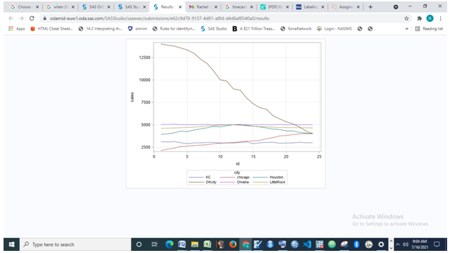
Fig 2: Time series plot
The descriptive statistics for auto sales are presented in fig 3. The result shows that OK city has the highest average sales (M=9117.71) while Kansas City has the lowest average sales (M=3015.42). sales variation is highest in OK city (sd=3481.67) while it is the lowest in Omaha (sd=15.99).
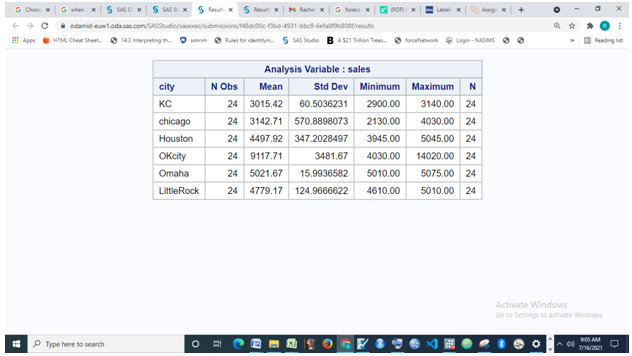
Fig 3: Descriptive Statistics
Regression Model
The study followed a step-by-step approach to arrive at the best model. The initial model analyzed is
sales=α_0+α_1 Trend+β_i city+γ_i season
After running the regression, we checked for the diagnostic test and found that the model is autocorrelated seen from the ACF plot in fig 4. We expect the bars of the ACF plot to be within the confidence bound but the first five bars are outside the bound. Therefore, we adjust the model by adding the first lag of sales.
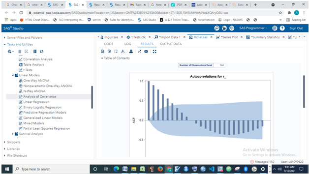
Fig 4: ACF plot
The new model is shown below
sales_t=α_0+α_1 Trend+α_2 sales_(t-1)+β_i city+γ_i season
The ACF plot of the residuals from the new model is presented in figure 5. The result shows that none of the ACF plots falls significantly outside the confidence bad. Thus, the model satisfies the assumption of no autocorrelation.
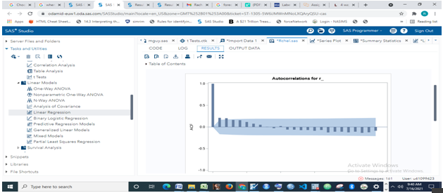
Fig 5: ACF plot of residuals for model 2
Other diagnostic plots are presented in fig 6. The plot of residuals versus fitted plot shows that linearity assumption was met moreover; we can also deduce that there is no heteroscedasticity from the same plot.
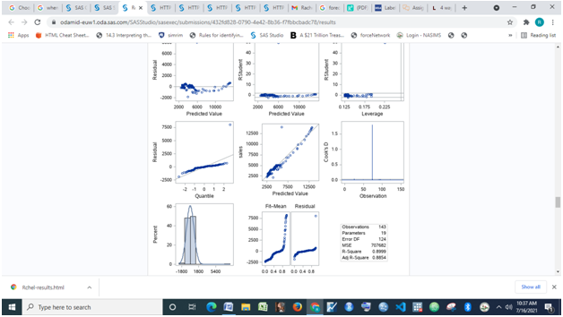
Fig 6: Residual Diagnostic plot
Regression Result
Fig 7 presents the regression result. The result shows that the trend (id) is significant in the model (p=0.0287). the coefficient is -26.77 which means that for every additional month auto sales decreased by approximately 27 cars. This means we will reject the null hypothesis (H0¬3) which connotes auto sales
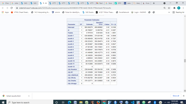
Fig 7:regression result
has a significant downward trend. Past month sales are positive and significant (beta=0.79, p<.001). This connotes the rejection of null hypothesis H01. Thus, a unit increase in last period sales increases present period sales by approximately 1 unit. None of the monthly dummies is significant (p>.05) which means there is no significant seasonality in sales. Moreover, only OK city sales are significantly different from the base, which is Chicago, the estimated coefficient of 1176.59 suggests OKcity average sales are higher than Chicago sales by approximately 1177 units.
The R2 of the model is 0.8854 which means the independent variables explain 88.54% of the variation in auto sales. Similarly, F(18,124)=61.96, p<.001 suggests the overall model is significant. This fact coupled with the diagnostic shows the model is sufficient to forecast future sales.
Forecast
The forecast for the next three months is presented in fig 8. The result shows that the sales for Kansas city are projected to fall for the next three months. It was projected to fall from approximately 3216 units in the first month to 2586 units in the second month and 2102 units in the third month. The same projection was made for Houston as it falls from 4255 units to 3638 units and further to 3166 units. Similarly, Little Rock Omaha and Chicago are predicted to witness a similar downward trend. The only OK city was forecasted to have increased sales from 5139 units to 4449 units and 3920 units in the third month.
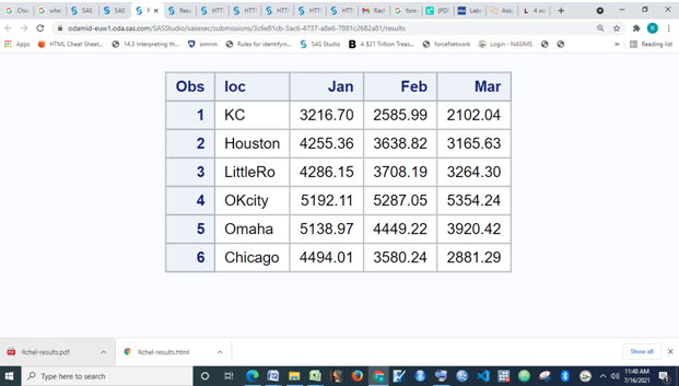
Fig 8: Forecasted Sales
CONCLUSION
The study has forecasted the next three months' sales of automobiles for six locations using a regression model. the step-by-step approach was followed in adding variables to the model. The result shows that a significant downward trend exists in auto sales. Previous period sales also affect present period sales while auto sales data do not exhibit seasonality. Five of the six locations are predicted to gave fallen sales over the next three months. The business insight from this analysis is that the managers can expect higher sales this month if last month's sales are high. Moreover, the management needs to take necessary steps to curb the predicted downfall in sales in the five locations where falling sales are predicted.