-
Homepage
-
Insurance Premium Homework Help
Computing Insurance Premium Payments Using R
Premium paid by the customer is the major revenue source for insurance companies. Default in premium payments results in significant revenue losses and hence insurance companies would like to know upfront which type of customers would default premium payments. The objective of this project is to predict the probability that a customer will default the premium payment, so that the insurance agent can proactively reach out to the policy holder to follow up for the payment of premium.
The customer fixation has contributed to a volatile property and consumer market. Turnover rates for consumers are historically high. Underwriting profit and consumer retention are becoming increasingly relevant in a tougher financial and economic environment. The days when ample earnings could be made on premium investments alone are gone. The combination of a volatile market for consumers and a greater emphasis on in portfolio management and development, underwriting needs a higher level of intelligence. The goal should be to aggressively search out groups of new customers who can and should be added to the portfolio, as well as to perform up-selling activities most likely to respond to current customers and with the greatest likelihood of future profitability.
Data Report
The data for this study were collected in both continuous and categorical forms. The continuous variables present in this study includes; Age of customers which is given in days, the income of customers, risk scores of customers, percentage of premium which were paid by cash and number of premium paid till date. Some of the categorical variables present in this study include marital status, type of residence area, sourcing channels among others.
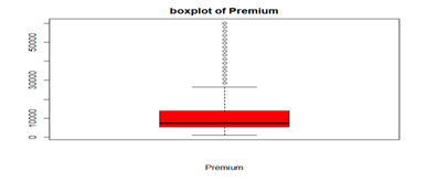
Figure 1: Boxplot of number of premiums
Figure 1 below above visualizes the variable number of premium. From the graph above, we can conclude there is no outlier present in the variable.
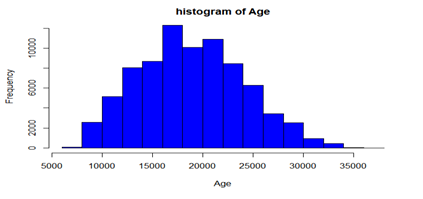
Fig 2: Histogram distribution of Age
Figure 2 above visualizes the age of customers in days and from the graph above we can conclude the age of customers were skewed to the right.
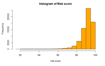
Fig 3: Histogram of risk score.
Figure 3 above visualizes the risk score of customers using the histogram chart and from the chart above we can conclude the risk score is skewed to the right.
Exploratory Data Analysis
Table 1 below shows the descriptive statistics of five continuous variables in this study using the mean and median as measure of central tendency. The Standard deviation as measure of dispersion and uses the skewness and kurtosis to measure the skewdness of each variable.
Age of customers has a mean of 188846.7, standard deviation of 520872 and positively skewed. Premium has a mean of 10924.51, standard deviation value of 9401.68 and positively skewed. Income has a mean value of 208847.2, a standard deviation value of 496582.6 and positively skewed. Furthermore, risk score has a mean value of 99.06, a standard deviation value of 0.73 and also positively skewed. Lastly, percent premium paid has a mean value of 0.31, a standard deviation value of 0.33 and positively skewed.
Table 1: Descriptive statistics of continuous variables
| Variable |
Mean |
Median |
S.D |
Skewness |
Kurtosis |
| premium |
10924.51 |
7500 |
9401.68 |
1200 |
60000 |
| Age |
18846.7 |
18625 |
520872 |
7670 |
37602 |
| Income |
208847.2 |
166560 |
496582.6 |
24030 |
90262600 |
| Risk score |
99.07 |
99.18 |
0.73 |
91.9 |
99.89 |
| Percent premium paid |
0.31 |
0.17 |
0.33 |
0 |
1 |
Table 2 below show the frequency distribution of some categorical variables present in this study. From the table below we found that 40032 unmarried customers and 39821 married customers were present in the study. 31670 customers live in the rural area while 48183 live in the urban area. 43134 customers were sourced through channel A, while 609 customers were sourced through channel E.
Table 2: Frequency distribution of categorical variables
| Variable |
Frequency |
Percentage |
| Marital Status
Unmarried
Married |
40032
39821 |
50.13
49.87 |
| Type of residence area
Rural
Urban |
31670
48183 |
39.66
60.34 |
| Sourcing Channels
Channel A
Channel B
Channel C
Channel D
Channel E |
43134
16512
12039
7559
609 |
54.01
20.68
15.07
0.95
0.08 |
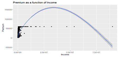
Bivariate relationship between premium and Income
This segment tests the relationship between number of premium and income of customers in the study using the scatter plots below to explain the relationship between them. From the graph below, a positive relationship between both variables premium and income was observed. Also the correlation matrix below in table 3 shows that a low positive correlation was found between both variables with correlation coefficient (r=0.3028).
Fig 4: Scatter plots between Income and Premium.
Table 3: Correlation matrix between premium and income.
| Variable |
Premium |
Income |
| Premium |
1 |
0.3028 |
| Income |
0.3028 |
1 |
Bivariate relationship between Age and Risk score
Lastly, this segment examines the relationship between age of customers and their risk scores. From the scatter plots in figure 5 below we conclude a positive relationship exist between both variables and from the correlation matrix in table 4 below a low positive correlation coefficient was found between both variables with (r=0.0479).
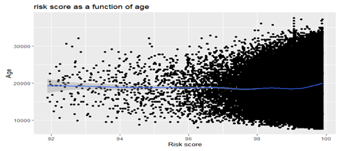
Fig 5: Scatter plots between age and risk score.
Table 4: Correlation matrix between Age and Risk scores.
Appendix (R Code)
| Variable |
Age |
Risk scores |
| Age |
1 |
0.0479 |
| Risk scores |
0.0479 |
1 |
Import dataset into R Environment
```{r setup, include=FALSE}
library(readxl)
Data <- read_excel("C:/Users/Admin/Downloads/Premium.xlsx")
head(Data)
str(Data)
```
transform data from character into factor form
```{r}
Data$residence_area_type<-as.factor(Data$residence_area_type)
Data$sourcing_channel<-as.numeric(Data$sourcing_channel)
Data$`Marital Status` <-as.numeric(Data$`Marital Status`)
```
Exploratory Data Analysis for continous variables
```{r}
boxplot(Data$premium, col ='red', xlab = 'Premium', main = "boxplot of Premium")
hist(Data$age_in_days, col ='Blue', xlab = 'Age', main = "histogram of Age")
hist(Data$risk_score, col ='Orange', xlab = 'Risk scores', main = "histogram of Risk score")
```
Summary/descritive statistics
```{r}
w = table(Data$`Marital Status`)
w
```
```{r}
X = table(Data$sourcing_channel)
X ```
```{r}
Y = table(Data$residence_area_type)
Y
```
```{r}
library(psych)
describe(Data$premium)
describe(Data$age_in_days)
describe(Data$Income)
describe(Data$risk_score)
describe(Data$perc_premium_paid_by_cash_credit)
```
Bivariate correlations between variables
Scatter plots between Income and premium
```{r}
library(ggplot2)
ggplot(Data, aes(x=Income, y=premium)) +
geom_point() + geom_smooth() +
ggtitle("Premium as a function of Income") +
xlab("Income") +
ylab("Premium")
```
Correlation between premium and income
```{r}
cor(Data$premium, Data$Income)
```