Histogram Approaches to Probability Density Functions and Probability Mass Function
This project will explore how a histogram approaches a probability density function (pdf or PDF) or a probability mass function (pmf or PMF) for a random variable and illustrate how to use the pmf/pdf to compute probabilities.
HISTOGRAMS, PDFS AND PMFS
By now, you should all know about histograms, after all, we discussed them in ENES101. We take a large collection events from multiple independent repetitions of a specific experiment, assign numbers to those events by means of a random variable, and then sort the values of the random variable into bins, counting the number in each bin. If we divide the number in each bin (i.e., the value of the histogram in that bin) by the total number of independent trials, we form a naïve estimate of the probability that the value of the random variable falls in that bin. Clearly, if we sum up all of these estimates, we should compute exactly 1.000…, because we will have accounted for all of the trials. Thus, in a simple view, the scaled histogram represents the scaled probability density function (if the random variable is continuous) or the probability mass function ( if the random variable is discrete). As the number of trials increases, the histogram should more and more closely approach the analytical pdf or the analytical pmf , where and represent the center of the bin.
PMF for a single fair die
Using the MATLAB function randi(imax, m, n) , model the number of dots showing on a fair six-sided die. In this case the number of dots – that is, resulting random integer – is the random variable. Each element of the returned matrix of values is one trial. Generate histograms using 120; 1200; 12,000; 120,000 trials and generate the scaled histogram, as described above. In each case, compute the (sample) mean and (sample) variance of your trials.
For those programming in a language other than MATLAB, randi(imax, m, n) creates an array of random integers in the range of 1 to imax.
Hint: use the appropriate MATLAB functions for this! Discuss your observations as the number of points increases. How do the histograms vary (or not) from what you expect. As shown in the figure 1 to figure 4, by increasing the trial, the mean and variance values is fitted to the expected values.
Comparing Sample Mean and Variance with Analytical Values
For this problem, the analytical expected value, or mean, is , and the analytical variance 2.9167. How do the (sample) mean and (sample) variance compare with the analytical values?
As Figure 4 shows, with 120000 trial, the mean and variance is calculated 0.166 and 2.9228 which is in accordance with the analytical values.
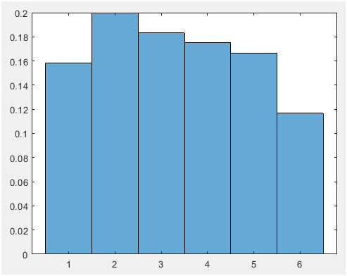
Figure 1. 120 trial (mean=0.166 and vaiance=2.6048)
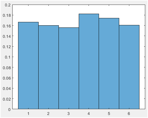
Figure 2. 1200 trial (mean=0.166 and vaiance=3.0075)
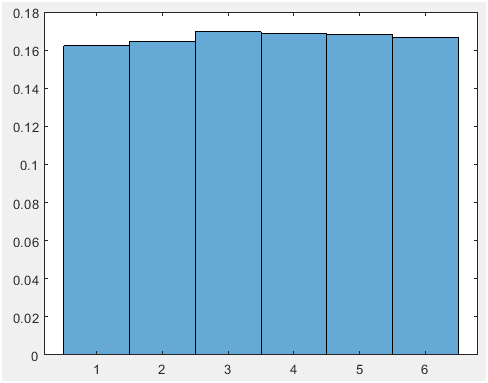
Figure 3. 12000 trial (mean=0.166 and vaiance=2.9159)
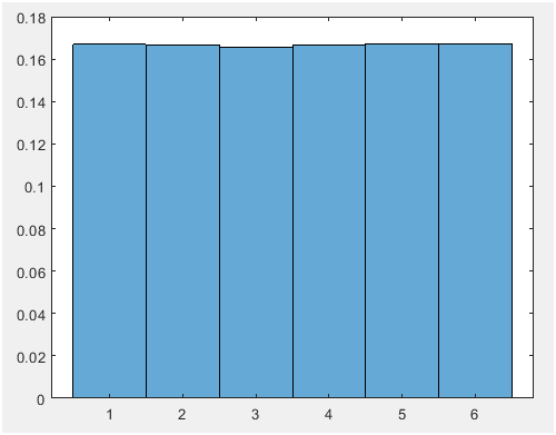
Figure 4. 120000 trial (mean=0.166 and vaiance=2.9228)
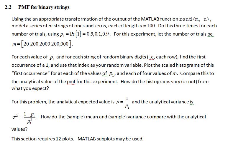
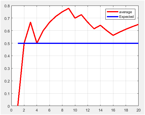
Figure 5. P1=0.5 and m=20
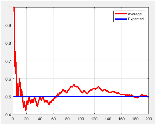
Figure 6. P1=0.5 and m=200
Figure 7. P1=0.5 and m=2000
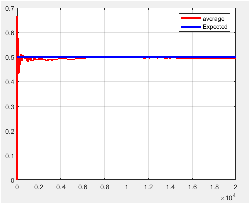
Figure 8. P1=0.5 and m=20000
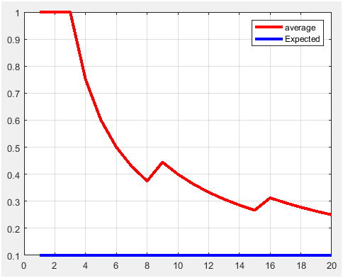
Figure 9. P1=0.1 and m=20
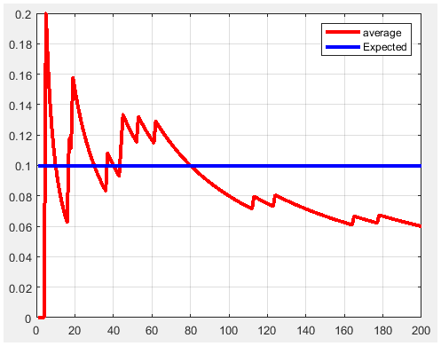
Figure 10. P1=0.1 and m=200
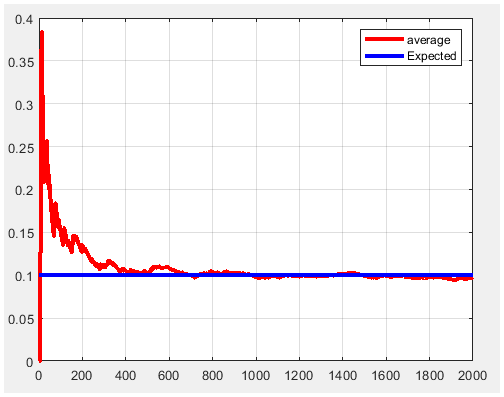
Figure 11. P1=0.1 and m=2000
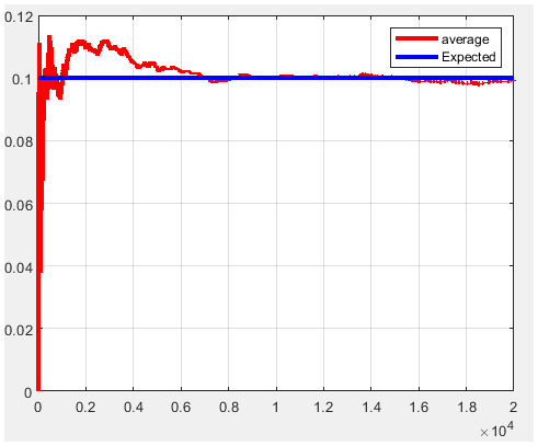
Figure 12. P1=0.1 and m=20000
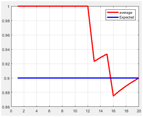
Figure 13. P1=0.9 and m=20
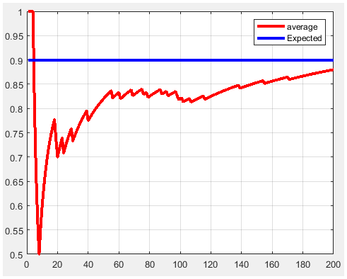
Figure 14. P1=0.9 and m=200
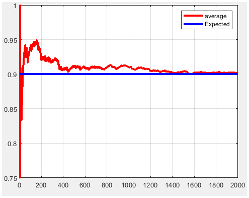
Figure 15. P1=0.9 and m=2000
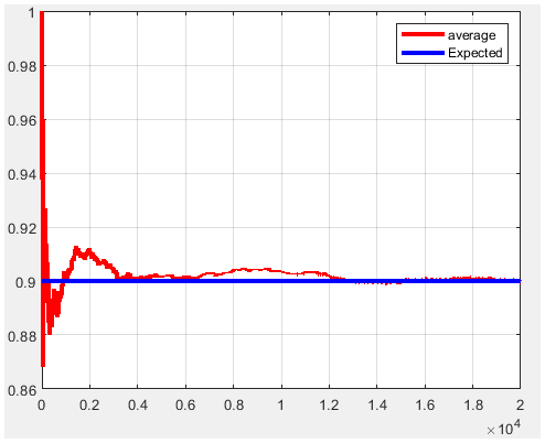
Figure 16. P1=0.9 and m=20000
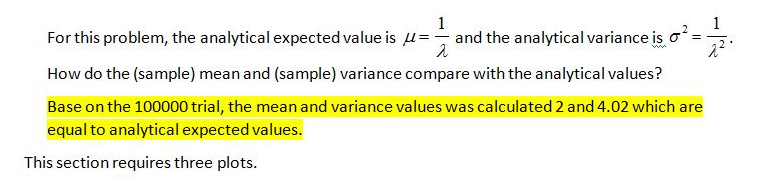
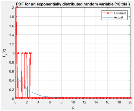
Figure 17.exponentially distribution with10 trial
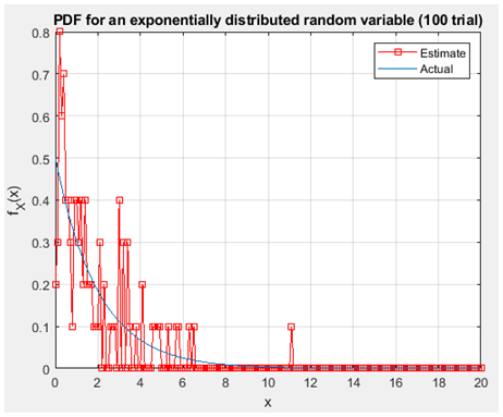
Figure 18.exponentially distribution with100trial
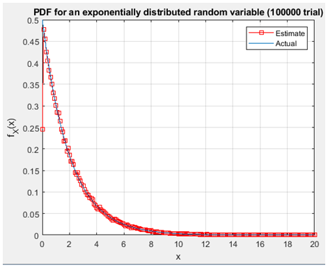
Figure 19. exponentially distribution with 1000000 trial
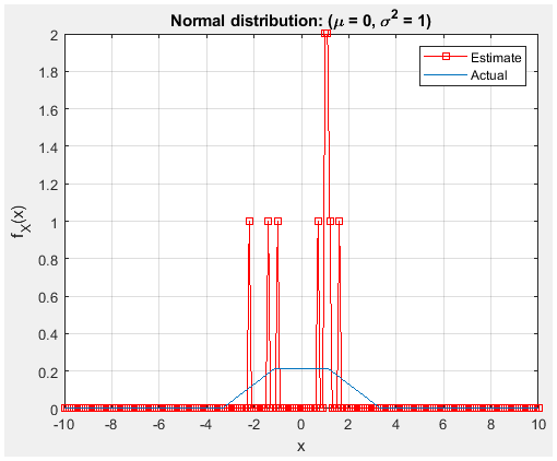
Figure 20. with 10 trial
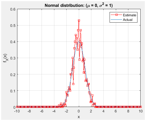
Figure 21. with 100 trial
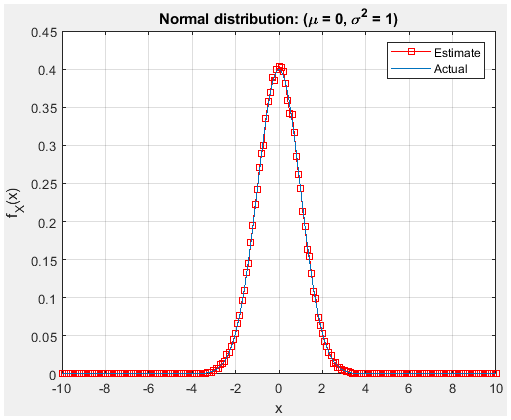
Figure 22. with 100000 trial
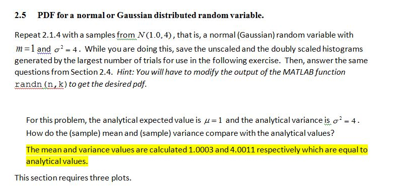
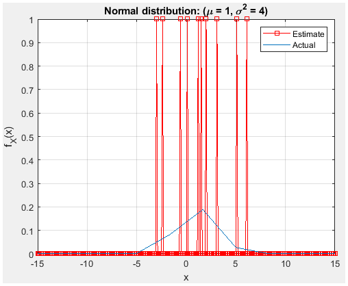
Figure 23. with 10 trial
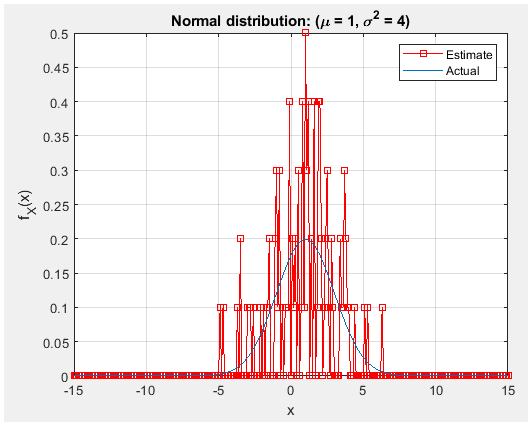
Figure 24. with 100 trial
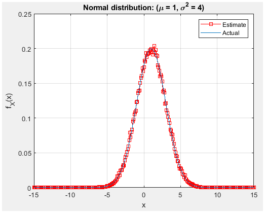
Figure 25. with 100000 trial
Figure 26.