Relationship between the age and relationship of a used Corolla
The solution below is based on MiniTab explaining the relationship between used Toyota Corolla, their age, and price. The solution involves identifying the right linear model.
Question
Classified ads at www.auto123.com (on July 22, 2013) offered used Toyota Corollas for sale in central Ontario. Some of the prices and age of the Corolla CEs with automatic transmission are found in the table below (data: Age vs Price).
| Age (Years) | Price ($) |
| 1 | 13900 |
| 1 | 14610 |
| 2 | 13998 |
| 2 | 16887 |
| 3 | 10900 |
| 3 | 12995 |
| 3 | 14995 |
| 4 | 10995 |
| 4 | 11998 |
| 4 | 11995 |
| 4 | 12495 |
| 5 | 8988 |
| 5 | 9488 |
| 5 | 10488 |
| 5 | 10989 |
| 7 | 11400 |
| 8 | 6995 |
| 9 | 6988 |
| 10 | 10000 |
| 12 | 2700 |
Solution
a) Provide a fitted line plot for these data and describe the association between age and price of a used Corolla.
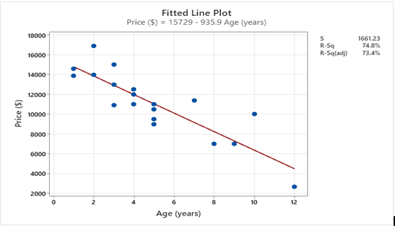
b) Do you think a linear model is appropriate?
Ans: Yes, it’s appropriate. The scatterplot depicts a linear relationship.
c) What is the equation for the line of best fit?
Ans: The regression equation isPrice ($) = 15729 - 935.9 Age (years)
d) What is the meaning of the value for the slope?
Ans: With every year increase in age, the price of the corolla tends to decrease by $935.9.
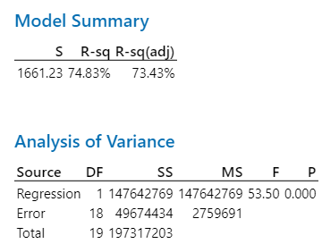
e) What is the residual standard deviation and what does it tell you?
Ans: The Residual Standard Error is the average amount that the response will deviate from the true regression line. Here the residual standard error is 1661.32.
f) What is the R2 and what does it tell you?
Ans: Here the R2 is 74.83%, which means that the linear model explains 74.83% variation in the Price.
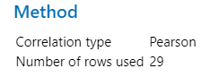
g) What is the Pearson correlation coefficient, and how is it related to R2?
Ans: The Pearson correlation coefficient represents the strength of the linear relationship between the two variables. It’s the square root of R2.
h) If you want to sell a 5-year-old Toyota Corolla, what price seems appropriate to ask?
Ans: The appropriate price is: 15729 - 935.9*5 = 11049.5.
i) You have a chance to buy one of two cars. They are about the same age and appear to be in equally good condition. Would you rather buy the one with the positive residual or the negative residual? Explain.
Ans: I would buy the one with the negative residual as it will have a lower price.
j) Why doesn’t this model explain 100% of the variability in the price of a used Corolla?
Ans: For that to happen the linear relationship should be perfect.
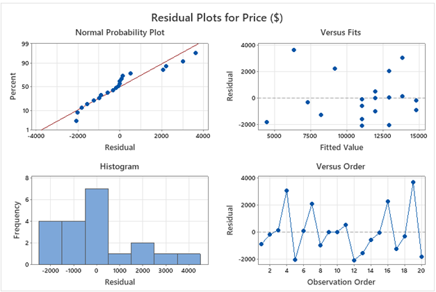
k) Check the residuals by obtaining a four-in-one plot. What can you say about the normality of the residuals? About equal variance assumption? About independence assumption?
Ans: From the graph, we can’t say that the residuals have normality. Equal variance and independence assumptions are seemed to be followed.
l) You see a “For Sale” sign on a 4-year-old Toyota Corolla with an asking price of $12000. What is the residual?
Ans: The predicted price for the Corolla is 15729 - 935.9*4 = $11985.4. Thus, the residual is $12,000-$11,985.4 = $14.6.
m) Would this regression model be useful in establishing a fair price for an 18-yr old Corolla? Explain.
Ans: No, it wouldn’t be good as 18 is out of the range of the observed values.
Remaining Minitab results:
Question
A materials engineer at a furniture manufacturing site wants to assess the stiffness of the particle board that the manufacturer uses. The engineer collects stiffness data from particle board pieces that have various densities at different temperatures. Data are found in the file Particle Board Stiffness.
Comparison between particle board stiffness and temperature
In this section, we used different methods such as Pearson correlations and MiniTab to determine the relationship between temperature and board stiffness.
a) What hypothesis should be run to determine if there is a significant association between stiffness and temperature?
Ans: We should use Pearson correlations, as the data are continuous.
b) Run the appropriate test in Minitab and show outputs.
Ans:
c) State your conclusions about the strength of this relationship if we use a 5% level of significance.
Ans: If we use a 5% significance level then, we don’t have sufficient evidence to support the claim that the two variables are correlated. This is because the confidence interval contains 0.
d) Are these conclusions supported by the R2 value for this relationship? Explain.
Ans: The R2 value is close to 0, thus it indicates our analysis is correct.
Question
Use the same data set for particleboard stiffness as in question 2
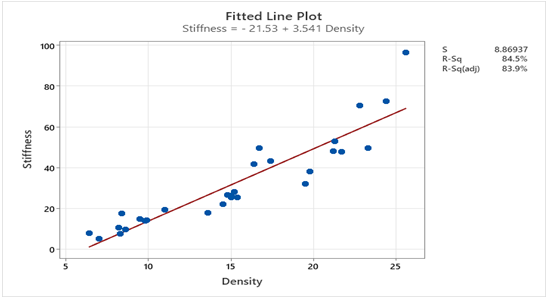
a) Obtain a fitted line plot from Minitab assuming we are trying to predict the stiffness of the particleboard from its density. Comment on the relationship you see.
Ans: The linear relationship here seems to be very strong.
State the hypothesis we should use to determine if there is an association between these variables.
Ans: We should test the hypothesis that H_0:β=0 vs H_1: β≠0, where β is the slope of the line.
Run the appropriate test in Minitab and show outputs.
Ans: The result obtained is:
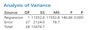
d) State your conclusions about the strength of this relationship if we use a 5% level of significance.
Ans: As the p-value of the test is significant, we can conclude that there’s a significant association between the two variables.
e) Are the assumptions satisfied? Provide appropriate plots to prove it and comment on what the plots show you.
Ans: The plots are:
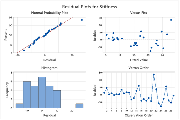
This shows that the assumptions of normality, equal variance, and independent samples are satisfied.
f) Calculate a 95% confidence on the slope of the regression line and interpret what it means.
Ans: The obtained result for the model is:
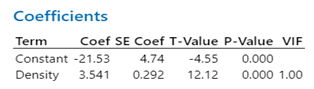
Using the above result we know that the SE of the slope is 0.292. Thus the 95% confidence interval is: 3.541±t_0.025,27*SE=3.541±2.052*0.292=(2.94,4.14). Interpretation: One can be 95% confident the per unit increase in density will increase the stiffness between the confidence interval.
Obtain from Minitab a 95% confidence interval on the average stiffness at a density of 8.5 and explain what the interval means.
Ans:
Obtain from Minitab a 95% prediction interval on the stiffness of a run of particle board for which its density is 7.8, and explain what the interval means.
Question
An automotive parts supplier assesses the usability and quality of the door locks that they provide. The locks are manufactured at three different plants. The production manager wants to determine whether the plant affects the final product. The production manager collects data on locks from each plant and gives a usability and quality rating. Data are found in the file Car Lock Ratings.
Use of the hypothesis to check the usability and quality of door locks
In this solution, we will run a one-way ANOVA in Minitab to compare the quality of door locks produced in three different factories.
a) State the null and alternate hypothesis we would run to determine if the Usability rating across all three manufacturing plants is the same.
Ans: Ho: The Usability rating across all three manufacturing plants is the same.
H1: The usability rating is different for at least one pair
b) Run a one-way ANOVA on these data in Minitab and show outputs.
Ans: The outputs:
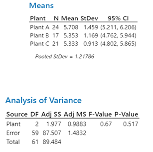
c) What conclusions can you make based on the p-value of this test?
Ans: The p-value is not significant thus; we can conclude that there’s not enough evidence to reject the claim that means the Usability rating across all three manufacturing plants is the same.
d) Obtain boxplot, residual plot, and residuals Normal distribution plots for these data set.
Ans: Boxplot:
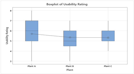
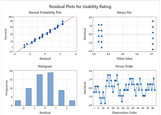
e) Have all assumptions been met? Explain using your plots to illustrate your answer.
Ans: The normality assumption is met as the probability plot shows a straight-line behavior from the residuals. Also, the variation seems to be equal in all the groups.
Question
A plant fertilizer manufacturer wants to develop a formula of fertilizer that yields the most increase in the height of plants. To test fertilizer formulas, a scientist prepares three groups of 50 identical seedlings: a control group with no fertilizer, a group with the manufacturer's fertilizer, named GrowFast, and a group with fertilizer named SuperPlant from a competing manufacturer. After the plants are in a controlled greenhouse environment for three months, the scientist measures the plants' heights. Data are found in the file Fertilizer – Plant growth.
a) State the null and alternate hypothesis we would run to determine if the average height of the plants is the same for all three fertilizer treatments.
Ans: Ho: The average height of the plants is the same for all three fertilizer treatments
H1: The average height of the plants is not the same for all three fertilizer treatments
b) Run the appropriate test in Minitab and show output. What conclusions can you make?
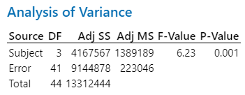
Ans: The ANOVA results:
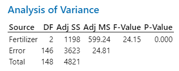
Using the output we can say that there’s enough evidence to reject the claim that the average height of the plants is the same for all three fertilizer treatments.
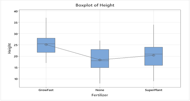
c) Obtain boxplots and residual plots for these data.
Ans: Boxplot:
Residual plots:
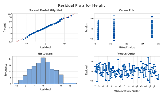
d) Are the assumptions of an ANOVA reasonably satisfied? Explain in reference to the plots.
Ans: Yes, the normality, equal variance assumption is looking fine. As the normal probability plot shows a linear trend while the deviation among the residuals seems equal.
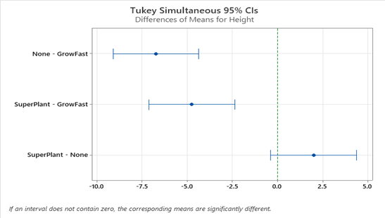
e) If there is a difference in the height by fertilizer treatment run a Tukey’s test to prove how the fertilizers compare to each other. Describe what the results of Tukey’s test tell you. Is there a fertilizer that is the optimum for plant height and if so, which one is it?
Ans: Using the graph we can say that there’s a difference in mean for Super plant-None with both None- Growfast and Super plant-Grow fast:
Question
A researcher investigates the factors that are associated with the salaries of professors who teach courses at a major university. The researcher gathers data about the subject area and the salary per course for a random sample of professors. Data are found in the file Academic Salaries by Subject Area.
Factors associated with the salaries of professors
In this solution, we are going to check the different factors that are used to pay professors at major universities. We will run a Minitab and also state the null and alternative hypotheses.
a) State the null and alternate hypothesis we would run to determine if the average salaries of the professors are the same across all subject areas.
Ans: Ho: The average salaries of the professors is the same across all subject area
H1: There is a difference in average salary for at least two subject areas among the professors
b) Run the appropriate test in Minitab and show output. What conclusions can you make?
Ans: The output:
We conclude that there’s sufficient evidence to reject the claim that the average salary for professors for different subject areas is not the same.
c) Obtain boxplots for these data, each individual data normality test plot, and one Normality plot for all residuals.
Ans: Boxplot:
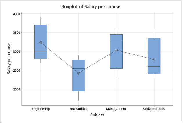
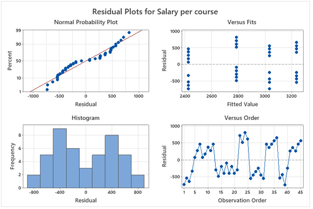
d) Are the assumptions of an ANOVA reasonably satisfied? Explain in reference to the plots.
Ans: The normality assumption doesn’t seem to be satisfied as it’s evident from the histography, which is bimodal. Also, using the Normal probability plot we can see that there’s no significant linear graph obtained.
e) If there is a difference in salaries run a Tukey’s test to show how the salaries for the different subject areas compare to each other. Describe what the results of Tukey’s test tell you.
Ans: Tukey results:
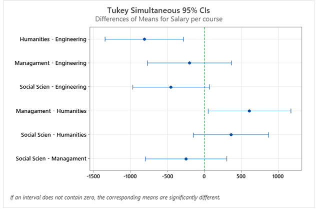

Using the two results, we can say that there’s a difference in mean between Humanities and Management, also between Humanities and Social sciences.