carrying out linear regression analysis using JMP
Here, we will carry out JMP to check whether teen births are associated with poverty, whether cigarettes affect the date of death and whether SAT scores can help predict college grades using GPA.
Task
As part of project 2, you will find 3 sets of bivariate data and 3 sets of data with 2 or more independent variables. You must select 3 data sets using at least one multiple regression data set.
The instructions for using JMP are covered in another document.
Each data set is in Excel. You should be able to import this information into JMP.
For the bivariate data sets, use JMP to create a scatter plot, compute the regression line, the model ANOVA, r2, and the parameter estimates. Provide copies of these printouts. In addition, provide a brief summary of what you see. The summary should be roughly 1 page in length for each analysis.
If you believe the relationship is not linear, you are NOT required to perform any transformation.
These data sets are:
- Cricket Chirping - Does the chirp rate of crickets change with temperature? Here is some data to see.
- Cigarette Smokers - These data represent a history of 15 smokers and their age at death.
- Teen Birth – This is the level of teen births related to the poverty level. This data provide percent of teens living in poverty and the birthrate per 1000.
For data sets with two or more independent variables, conduct a multiple regression using JMP. Provide the final regression model, r2, the model ANOVA, and the parameter estimates. Provide copies of these printouts. In addition, provide a brief summary of what you see. Of particular note would be which independent variables to keep and which to ignore. That may mean running the analysis more than once.
Unless already given in the data, you do NOT have to consider any interactions, polynomial terms, or other transformations in the analysis, although appropriate comments may be given.
- Plants2 - Two Species of plants by 7 levels of watering. Look at both the wet and dry biomass as a function of watering and plant type. 0=Leucaena, 1=Accacia
- Majors – Can SAT scores predict success in college based on GPA. This group includes two majors, 0-Computer Science, 1-Engineering.
- Car Tire Properties – Which of the 4 properties of rubber used in car tires is influenced by 3 key chemical components?
Solution
Is the level of teen births related to the poverty level?
The simple linear regression model has been built for teen births using the percent of teens living in poverty as the explanatory variable. The regression model has been created using the Ordinary least square method which is aimed at minimizing the sum of squared residuals using JMP software.
To explore the relationship, the scatter plot between the two variables is created and presented in Figure 1. It can be clearly seen that the trend is upward sloping suggesting that the higher the poverty level, the higher is the number of teen births, and vice versa. And the relationship from the scatter plot looks quite strong.
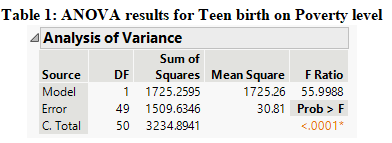
The ANOVA results from the regression model presented in Table 1 under the null hypothesis which states that teen births are not related to poverty level and the alternate hypothesis states that teen births are related to poverty level shows that the value of the F-stat at 1 and 49 degrees of freedom is 56 with its p-value close to zero. Since the p-value is less than 0.01 at the 1% alpha level, we have enough evidence to reject the null hypothesis and it can be concluded that teen births are related to the poverty level.
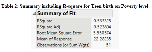
Furthermore, it can be seen that the value of R-square in Table 2 is 0.5333 which means that about 53.33% of the variation in teen births is explained by poverty level and it can be considered to be a good fit model.
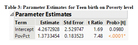
Furthermore, the regression line that is predicted using the data from Figure 2 can be written as follows:
Teen Birth = 4.267 + 1.373*Poverty level
The value of the slope at 1.373 suggests that an increase in the percent of teens living in poverty by 1% results in about 1.37 more teen births per 1000. And the value of intercept at 4.267 suggests that if the poverty level is zero percent, there are on an average of 4.267 teen births per 1000.
Thus, it can be concluded from the above analysis, that teen birth is related to the poverty level.
JMP Output
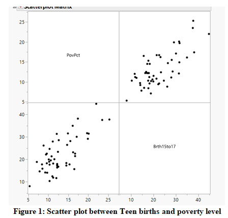
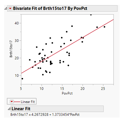
Figure 2: Regression Line for Teen birth on Poverty level
Does the number of cigarettes smoke per day influences age at death?
The simple linear regression model has been built for age at death using the number of cigarettes smoked per day as the explanatory variable. The regression model has been created using the Ordinary least square method which is aimed at minimizing the sum of squared residuals using JMP software.
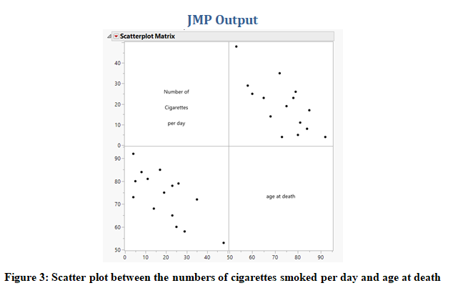
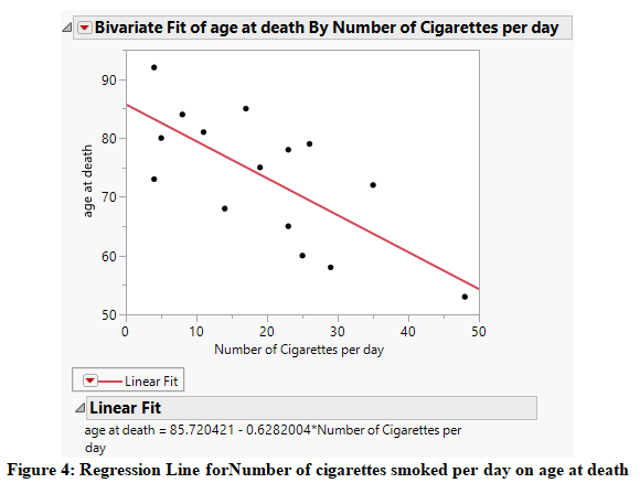
To explore the relationship, the scatter plot between the two variables is created and presented in Figure 3. It can be clearly seen that the trend is downward sloping suggesting that the higher the number of cigarettes smoked per day, the lower is the age at death and vice versa. And the relationship from the scatter plot looks quite strong.
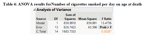
The ANOVA results from the regression model presented in Table 4 under the null hypothesis which states that the number of cigarettes smoked per day is not related to age at death and the alternate hypothesis states that the number of cigarettes smoked per day is related to age at death shows that the value of the F-stat at 1 and 13 degrees of freedom is 13.48 with its p-value of 0.0028. Since the p-value is less than 0.01 at the 1% alpha level, we have enough evidence to reject the null hypothesis and it can be concluded that the number of cigarettes smoked per day is related to age at death.
Furthermore, it can be seen that the value of R-square in Table 5 is 0.50898 which means that about 50.9% of the variation in age at death is explained by the number of cigarettes smoked per day and it can be considered to be a good fit model.
Furthermore, the regression line that is predicted using the data from Figure 4 can be written as follows:
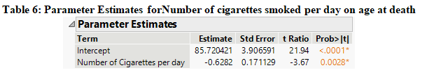
Age at Death = 85.72– 0.628*Number of cigarettes smoked per day
The value of the slope at 0.628 suggests that every unit increase in the number of cigarettes smoked per day results in a decrease in age by about 0.628 years. And the value of intercept at 85.72 suggests that if a person does not smoke any cigarettes per day, the average age of the person is 85.72 years.
Thus, it can be concluded from the above analysis, that age at death is related to the number of cigarettes smoked per day.

Can SAT scores predict success in college based on GPA?
The data set comprises of college GPA, SATM, and SATV along with the major which is a dichotomous variable with the value of 0 for Computer Science and 1 for Engineering. The multiple linear regression model has been built for success in college based on GPA using SATM, SATV, and major as the explanatory variables. The stepwise method of regression is used whereby the significant explanatory variables are included in the model step by step.
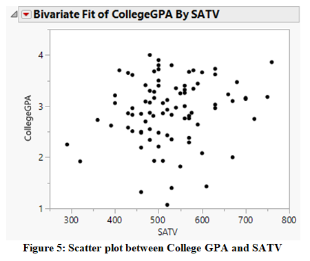
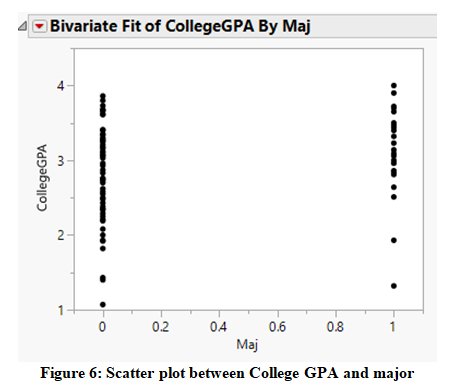
To explore the relationship, the scatter plot between the pairs of variables are created and presented in Figure 5 and 6. It can be clearly seen in Figure 5 that the trend is upward sloping between College GPA and SATV suggesting that the higher the SATV, the higher is the college GPA, and vice versa. And the relationship from the scatter plot looks quite strong. Furthermore, Figure 6 showing the relationship between college GPA and major shows that the College GPA is comparatively higher in Engineering major than in Computer Science major. And the relationship from the scatter plot looks quite strong.
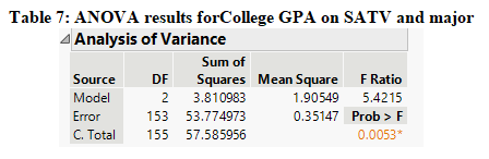
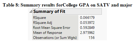
The ANOVA results from the regression model presented in Table 7 under the null hypothesis which states that none of the explanatory variables included in the model is related to success in college based on GPA and the alternate hypothesis states that at least one of the explanatory variables included in the model is related to success in college based on GPA, shows that the value of the F-stat at 2 and 153 degrees of freedom is 5.42 with its p-value of 0.0053. Since the p-value is less than 0.01 at 1% alpha level, we have enough evidence to reject the null hypothesis and it can be concluded that at least one of the explanatory variables included in the model is related to success in college based on GPA. Furthermore, it can be seen that the value of R-square in Table 8 is 0.066 which means that about 6.6% of the variation in college is explained by all the explanatory variables included in the model but since the value is quite low it cannot be considered to be a very good fit model.
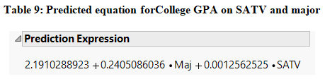
Furthermore, the regression line that is predicted using the data using stepwise regression includes two explanatory variables from Figure 9 can be written as follows:
College GPA = 2.19 + 0.24*Major + 0.00125*SATV
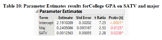
The value of slope for SATV at 0.00125 suggests that an increase in the one unit of SAT score in verbal results in about 0.00125highercollege GPA keeping major as constant. Also, the value of slope for Major at 0.24 suggests that on average the college GPA for Engineering students is 0.24 units higher than Computer Science students keeping SAT verbal score as constant.
Thus, it can be concluded from the above analysis, SAT verbal score and major are significant predictors for success in college while SAT score in Maths is not a significant predictor.
JMP Output