Interpretation of results based on Econometrics
Here, we will use econometrics to determine the number of salaries different people receives based on different circumstances.
QUESTIONS
Task A
Pick one of the available subjects in the data, and in no more than 100 words, explain your motivation on why you would like to use this subject as the comparison subject. Please also clearly indicate the word count within your answer. In addition, provide two tables of descriptive statistics for variables Salary, Male, Tariff, Age, Polar, Degree class, and Region, one for Economics graduates, and another one for the comparison subject. Note that you don’t need to provide the Stata commands used to obtain these descriptive statistics and you only need to show the mean and standard deviations (for the categorical variables you need to show the mean for each category). Based on these descriptive statistics, describe in no more than 300 words the main similarities/differences between the two subjects. Please also clearly indicate the word count within your answer.
Task B
Investigate the main question of the Project by using descriptive statistics only; e.g. by appropriate use of means, medians, standard deviations, interquartile ranges, etc. Your answer can also include appropriate graphs. Don’t forget that you need to investigate this for both subjects; i.e. for Economics and for the comparison subject. There is no word limit for this question, but your answer needs to be presented within two A4 sides (so, all tables, graphs, and discussions need to be presented within two A4 sides, i.e. one full page).
Task C
In this part, you need to investigate the main question of the Project by using regression analysis (i.e. appropriate MLR models). That is, you need to investigate whether Male graduates are expected to ‘earn more/less’ relative to Females and assess how big these differences are. Don’t forget that you need to investigate this separately for Economics and for the comparison subject. You also need to investigate this by first using Empty regression models (i.e. model that only includes that Male dummy variable), and then by using Full regression models (i.e. models that also include additional explanatory variables). That is, you will need four separate MLR models, an Empty and a Full for Economics graduates and an Empty and a Full model for the comparison subject. Here are some important further instructions/notes. Please read these very carefully:
(1) The dependent variable Salary must be used in the logarithmic form (i.e. the natural log of salary).
(2) In your discussion of the results of your regression models, you need to provide an appropriate interpretation of the coefficients associated with the Male dummy variable. You need to provide this interpretation both for the Empty and the Full models, and also provide a comparison between the two.
(3) You also need to conduct appropriate hypothesis testing, to test whether the gender pay gap is statistically different from 0. You need to provide this hypothesis testing both for the Empty and the Full models, and also provide a comparison between the two.
(4) It is up to you to decide which other explanatory variables you add to your Full models and that it is not necessary that the model set for Economics includes the same variables with the model set for the comparison subject. Note that categorical variables (such as degree class or region, need to include appropriate dummy variables for each category (excluding one to avoid perfect multicollinearity). For each explanatory variable that you include in the Full models, you need to offer a short justification on why it is important for these variables to be included in the model (max of 150 words for the justification of each variable). Note that you need to present a single justification for both ‘Economics’ and the ‘comparison subject’, instead of a 150 words justification for ‘Economics’ and then another 150 words just for the ‘comparison subject’. Similarly, for the variables that you decide not to add to your model, you also need to provide justification as to why these were not added (again a max of 150 words for each variable not added).
(5) Note that variables Tariff and Age must be included in the Full models, so please don’t provide justifications on why these variables are included in the models. Nevertheless:
– For Tariff, you need to decide whether you use it in its linear form, or whether you include a quadratic term / replace it with the natural log of Tariff. Your choices need to be justified within a max of 250 words.
– For variable Age, you need to decide whether you use it just in the linear form or whether you include the quadratic form too. You also need to provide two graphs for the predicted log of salary against Age, one for Economics and one for the comparison subject. Then, based on these graphs, you need to discuss the relationship between age and salary in the two. Your choice justification and the discussion of the graph should not exceed 350 words in total.
– Note that you are allowed to use different forms of Tariff and Age across Economics and the comparison subject Full models.
(6) Your Full regression models need to be tested for violation of MLR5 (i.e. whether there is a heteroskedasticity problem). If there is statistical evidence of heteroskedasticity, then the standard errors presented in your regressions must be made ‘robust to heteroskedasticity’. Also, if your model is made robust to heteroskedasticity, then note that the hypothesis testing, under point (3), needs to be done on the ‘robust’ models. Please note that testing for heteroskedasticity and correcting the standard errors are covered in the material of Week 12.
(7) Note that all your regression results need to be presented in one or two tables. There are Stata commands that create such tables automatically, such as the ‘outreg2’ command. This was discussed in the Support Session of Week 10 (an extract of the video recording where I discuss this, can also be found in the ‘Introduction to Stata Material’ section on the module’s BB). My suggestion is to have one table with 5 columns. A first column for the variables, two columns for the estimates of the ‘Economics’ models (one for the Empty and one for the Full model), and two columns for the estimates of the ‘comparison subject’ models (again, one for the Empty and one for the Full model).
Task D
Provide a short literature review of other academic papers that investigated a similar question (i.e. gender pay gaps). This review needs to be based on up to 5 academic references, and a list of these references needs to be provided at the end of your answer using a consistent referencing style. Note that these academic references can be either published papers in academic journals or other academic reports published by academic institutions (such as the Institute of Fiscal Studies). Newspaper articles are not valid academic references. The answer to this part must be contained within two sides of a page, i.e. one full page, including the 5 references. Within this review, also discuss whether the findings of these papers are similar or different from the ones you obtained in Task C.
Task E
Present the main findings of your regression analysis within a single graph. This graph needs to focus on the ‘gender pay gaps’ found in the regression analysis. Note that this can be a ‘combined graph’ and it can be produced either in Stata or in Excel. If the graph has been done in Stata, you don’t need to provide the required Stata command. Also, provide a discussion/summary of the findings presented in this graph and try to avoid using technical language (i.e. econometric terminology that would not make sense to a non-specialist). The answer to this part must be contained within one side of a page.
Task F
Only for the Economics regression model, in your Full model, add (an) interaction term(s) between the Male dummy variable and one of the explanatory variables. Estimate this model, present your results and provide a discussion of the additional insights obtained following the model with the interaction term(s). Note that for this part, you can just copy/paste the Stata output instead of creating your own table. Within your answer, you also need to justify why you have picked this explanatory variable for the interaction term(s). The answer to this part must be contained within two sides of a page, i.e. one full page.
Solution
Task A
The rationale for picking business/management as the comparison subject
The rationale between these selections is that both courses are similar in some respect. One, they are both concerned with resource allocation and getting the best possible result using the least possible resources. Second, they are studied in school for the same number of years. However, economics is wider in scope than business/management as economics look at the whole while business/management’s scope is limited to only the business world. Thus, it is necessary to determine if the wider scope results in higher pay for economics graduates.
Descriptive Statistics
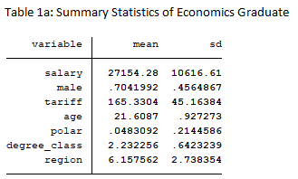
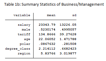
Table 1a and 1b presents the summary statistics for economics and business/management graduates respectively. The average salary for economics graduates is $27,154 which is greater than the average salary for business/management graduates at $23,343.79.Variation in salary is higher for business/management graduate (sd = 13,226.05) compare to economics graduate (sd = 10.616.61). The average value for the male variable is 0.7042 while for business/management graduates is 0.523. This means there is more proportion of males (70.42%) in economics than business/management (52.3%). UCAF tariff points are greater for economic students (mean=165.33) than their counterparts in business/management (M=134.87). The variation in tariff points also follows the mean (45.16 vs 39.28). The average age is closer between the two discipline although economics have a slightly younger age with lower variation (M=21.61 years, SD=0.97) than business/management (M=22.06 years, SD=1.47). For the polar variable, more proportion of business/management (8.68%) students grew up in a region with low participation neighborhood than economics graduate (4.83%). It appears that the majority of economics and business/management students have a second-class upper grade as the mean for both grades is close to 2 (2.23 for economics and 2.21 for business/management). Since second class upper is coded as 2, the mean is close to 2 means it dominates other classes of degrees.
In summary, the summary statistics showed that economics graduates earn more on average than their business/management counterparts. The proportion of male to female in economics course is higher than that of business/management. Similarly, the tariff point is higher for economics graduates than business/management graduates. More proportion of business/management students grew up in the region with low participation neighborhood than economics students. Second class upper grade dominate other grades for both subjects
TASK B
Before making the comparison of annual salary between males and females, it is appropriate to check the distribution of annual salary. If the distribution is normal, then it is appropriate to use the mean and standard deviation to compare annual salary between gender. Thus, we plotted the histogram of annual salary and imposed a normal density on it for data that incorporate both economics and business (Total) and separately for economics and business/management. The plot shows that the annual salary is positively skewed in all cases with a high peak for business data and a total and normal peak for economics. The result showed that the annual salary does not follow a normal distribution. Thus, we cannot use mean and standard deviation for comparison as they will be biased by extreme values present in the dataset.
Figure 2a: Histogram of Annual Salary
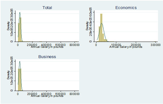
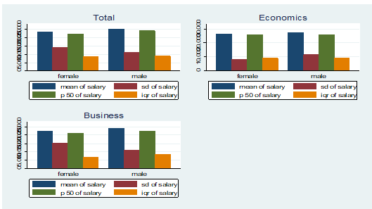
Table 2 presents summary statistics of annual salary by gender, the median and interquartile range as well as the mean and standard deviation. The result showed that the median annual salary is higher for males (Median=$24,000, IQR=$8875) than females (Median=$20,000, IQR=$8,000) in the total data. Similarly, the median annual salary is higher for males (Median=$22,150, IQR=$8500) than females (Median=$21,000, IQR=$8,000) among management/business graduates. However, as for Economics graduates, there is no difference in median annual salary between males and females as both median and IQR equals $26,000 and $9,000 respectively for both males and females. The result showed that while the gender gap was found for business graduates, there is no such gap for economics graduates. However, if we had made the decision with mean and standard deviation, we could have found a gender gap for both economics and business which means the mean has been biased by extreme values shown by the histogram. In conclusion, descriptive statistics suggest a gender gap for business/management graduates but not economics graduates.
Table 2: Summary statistics of annual salary by gender
| female Economics | Male economics | female business | male business | female total | male total | |
| mean | 26437.74 | 27455.27 | 22452.05 | 24157.03 | 21627.17 | 25284.81 |
| sd | 8161.74 | 11481.08 | 15262.76 | 10985.2 | 14648.12 | 11265.39 |
| p50 | 26000 | 26000 | 21000 | 22150 | 20000 | 24000 |
| iqr | 9000 | 9000 | 7000 | 8500 | 8000 | 8875 |
The result in the table is presented graphically using the bar chart in figure 2b
Figure 2b: Bar chart showing summary statistics of annual salary by gender
Code for this task
label define male 0 "female" 1 "male"
label values male male
tab male
bysort male: tabstat salary, statistics(mean sd median iqr) column(variable)
bysort male: tabstat salary if subject==1, statistics(mean sd median iqr) column(variable)
bysort male: tabstat salary if subject==5, statistics(mean sd median iqr) column(variable)
graph bar (mean) salary (sd) salary (median) salary (iqr) salary, over(male) name(Total,replace) title("Total")
graph bar (mean) salary (sd) salary (median) salary (iqr) salary if subject==1, over(male) name(Economics,replace) title("Economics")
graph bar (mean) salary (sd) salary (median) salary (iqr) salary if subject==5, over(male) name(Business,replace) title("Business")
graph combine Total Economics Business
histogram salary, normal title(Total) name(Total,replace)
histogram salary if subject==1, normal title(Economics) name(Economics,replace)
histogram salary if subject==5, normal title(Business) name(Business,replace)
graph combine Total Economics Business
TASK C
Variables included in the full model
Degree_class: the degree class is often associated with capabilities and intelligence which means a person with a higher degree class is perceived to have the high capability and intelligence than others with a low degree class. Thus, a person with a high degree class has a higher chance at a high-paying job where competition is very high.
Russell: some online surveys have shown that the universities attended have an impact on future earnings as they found that some universities graduate earn higher than other university graduates even though they studied the same course. For example, the survey cited that economics graduates from LSE earn on average $70,500 five years after graduating while their colleague from Cambridge University earns $77,900.
Joint: graduates with single honors have limited opportunities compared to their colleagues with double honors. Thus, a graduate with double honor may have the opportunity to the high-paying job just because the course required for the job is one of the honors while a single honor graduate may be denied high-paying job because his course is not required for the skill.
Variables not included
Region of Education: it is often said that talent is evenly distributed but opportunity is not. With the present globalization and civilization, other things being equal there is no region bias when seeking for job and no one can be denied high paying job because he schooled from one region.
Soceon_class: the parents’ socio-economic status may not affect pay since we are dealing with data on those who are graduated. Parents’ socioeconomic status may affect educational attainment but since we are considering those who graduated already, there is no need to include it in the model.
Polar: coming from low participation neighborhoods will not likely affect future payment for graduates as these are not considered as a requirement to participate in job interviews and graduates from low or high participation neighborhoods are not favored nor biased against during job interviews.
Justification for forms of age and tariff in the model
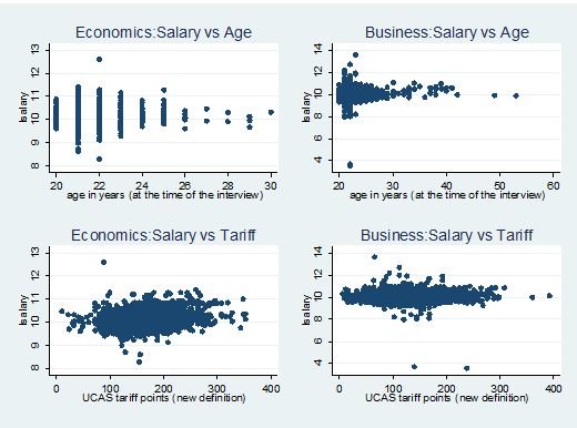
Figure 3a presents the scatter plot of salary against age. The plot shows that the pattern of relationship between age and salary is not clear from the plot which may be due to the limited range for age. However, the preliminary regression model shows that the square of age has a significant effect on the model. Thus we will use age in quadratic form. On the other hand, there is a clear linear relationship between salary and tariff but I prefer to use it in logarithm form in order to interpret the coefficient as elasticity.
Fig 3a: Scatter Plots
Heteroscedasticity Test
The heteroscedasticity test result for the four models is presented in table 3a. The result showed that for the four models, there is significant evidence of heteroscedasticity in the models as p<.05. Thus, we use robust standard errors for all the models.
Table 3a: heteroscedasticity Test
| empty economics | 10.81(0.001) |
| empty business | 5.20(0.023) |
| full economics | 7.28(0.007) |
| full business | 28.45(<.001) |
Regression Result
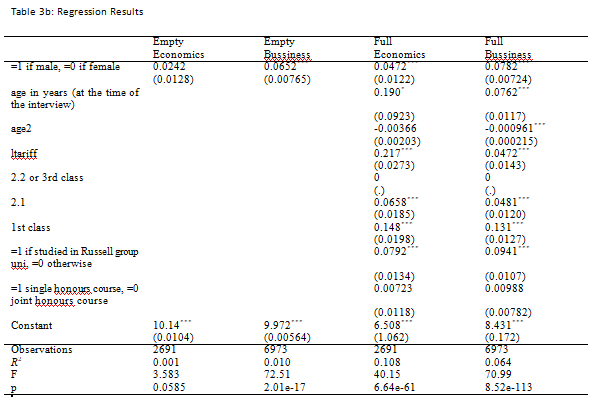
The full regression result is presented in table 3b. The empty model for economics graduates showed that the estimate for the dummy representing males is positive (beta=0.0242, se=0.013). However, the p-value is greater than 0.05 which is indicated by no star. On the other hand, when other variables are considered (full model), we see that the estimate of the dummy representing male is significant and the estimate doubled in size. Thus, considering the empty model, there is no gender pay gap among economics graduate even though male economics graduate earned on average 2.42% higher than their female counterpart but the full model confirm significant gender gap exists between economics graduate and male earning on average 4.72% higher than female. For business/management graduates, the estimate for males is statistically significant for both empty and full models. The empty model estimated coefficient is 0.0472 which means that on average, male salary for business graduates is 4.72% higher than female business graduates while for the full model the difference is as high as 7.82%.
Comparing economics and business, the gender gap is significantly present in both models but it is much higher among business graduates than economics graduates. Age and its squared term are significant for both economics and business models and the same is observed for tariff. First-class and second-class upper graduates have significantly higher salaries than second-class lower and third-class graduates. Moreover, those who studied in Russell group universities have significantly higher pay of 7.92% and 9.41% for economics and business respectively than those who studied in non-Russell group universities. There are no sign of double honors which means no significant pay gap between graduates who have double honors and single honors. The overall model is significant except for the empty model for economics graduates while the independent variables in the full model explained 10.8% and 6.4% of the variation in the salary for economics and business models respectively.
Code for Task C
twoway (scatter lsalary age if subject==1) , title(Economics:Salary vs Age) name(Economics,replace)
twoway (scatter lsalary age if subject==5) , title(Business:Salary vs Age) name(Business,replace)
twoway (scatter lsalary tariff if subject==1) , title(Economics:Salary vs Tariff) name(Ec,replace)
twoway (scatter lsalary tariff if subject==5) , title(Business:Salary vs Tariff) name(bs,replace)
graph combine Economics Business Ec bs

reg lsalary male if subject==1
hettest
reg lsalary male if subject==1,robust
reg lsalary male if subject==5
hettest
gen ltariff=log(tariff)
reg lsalary male age age2 ltariff i.degree_class russell joint if subject==1
hettest
reg lsalary male age age2 ltariff i.degree_class russell joint if subject==5
hettest
eststo: reg lsalary male if subject==1,robust
eststo: reg lsalary male if subject==5,robust
eststo:reg lsalary male age age2 ltariff i.degree_class russell joint if subject==1,robust
eststo:reg lsalary male age age2 ltariff i.degree_class russell joint if subject==5,robust
esttab using result.rtf,se r2 label replace nogap compress scalars(F p)
TASK D
The issue of the gender pay gap has been thoroughly discussed in the literature with some studies focusing on the issue broadly while others focused on a particular course of study. It is almost a unanimous result that there is a significant gender wage gap. Wood et al. (1993) studied the gender gap in pay among Michigan Law School graduates. The authors believed that both male and female law graduates have identical human capital although some factors like child care may cause a gap in payment. After controlling for such gaps, they found that 25% of the gender pay gap was not explained. Francessoni and Parey (2018) used data on six cohorts of University graduates in Germany to examine the extent of the gender gap in pay after twelve to eighteen months of graduation. They found that men and women are admitted to universities in roughly equal proportion. Moreover, females enter college with better high school grades but leave with a slightly lower grades. They found that even though men and women work for a similar number of weekly hours but men get higher pay than females. They conclude that the field of study in the university can explain the gap.
Noonan et al. (2005) used survey data from Michigan Law School graduates to compare the sex gap over time. They found that males earn 52% more than women but for those who have the same characteristics, the gap is 17% and if in addition, the job settings are the same the gender gap is 11%. Reiner and Schroder (2006) used data from Mannheim University Social Science Graduates to investigate gender pay gaps among graduates. The author includes measures of human capital with the result suggesting if human capital were equal for males and females, the pay gap would have been wider. Moreover, after controlling for some factors, the pay gap is still 7%. Livanos and Nunez (2012) used Labour Force Survey data for Greece and United Kingdom to analyze the gender wage gap using Oaxaca decomposition. They found that the gender gap related to discrimination reduces with a higher level of education. Comparing the surveyed studies with my result, my result is consistent with what has been found in the literature that a significant gender pay gap exists.
TASK E
Figure 5a: Gender Gap Visualization
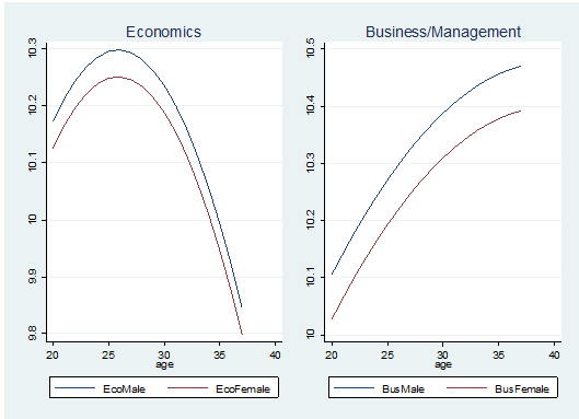
In order to make a visualization of the main findings, we made some assumptions. We consider male and female graduates of Economics and Business studies that both have the average tariff score, were both first-class graduates, both graduated from Russell University, and are both single honors, we now plot their predicted salary over the age range of 20-40. The plot revealed that the line for males for both business and economics is always above that of females which means there is always a gender pay gap between males and females for both business and economics graduates.
Task F
Table 6: Regression with Interaction of age and gender
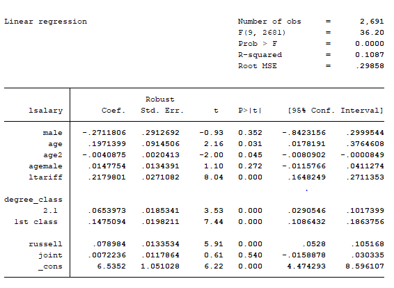
The regression result with the interaction of age and gender is presented in table 6. The choice of age is informed by the fact that as age advanced, the participants likely move to higher rank which results in a higher salary. However, if both genders have equal opportunities to hold the higher posts, it may mitigate some of the gender pay gaps that have been observed. If this is true, the estimated coefficient for the interaction term should be negative and significant. However, contrary to expectation the estimated coefficient is positive but insignificant. This means the gender pay gap between males and females does not vary across age. The estimated coefficient for male turned negative and insignificant but even if it is significant, it does not mean the table has turned and female are now earning higher than male as the interaction term still need to be considered because in this model
Even this equation is positive at the minimum value of age in the model which means the gender age gap still exists. The main conclusion here is that the gender wage gap does not differ across ages.
Code for this part
gen agemale=age*male
reg lsalary male age age2 agemale ltariff i.degree_class russell joint if subject==1,robust