Assignment instructions
- Open the Data set associated with Project Part I
- Create a table that lists each variable and its most likely level of measurement. Format the table to class expectations as required on ALL assignments.
- Generate an Excel descriptive statistic table for each variable. Discuss and report the measures of central tendency (mean and median), measures of variability (standard deviation, IQR, and range), kurtosis, and skewness numerical summaries. See the exemplar (posted at the top of the course list in Moodle) for a sample write-up. DO NOT JUST LIST the numerical summaries. Each of the numerical summary areas (measure of center, variability, kurtosis, and skewness) must have an associated meaningful interpretation to receive credit.
- Based on the descriptive statistic tables generated in #3 above, which is the better measure of the center (mean or median) for each variable? Justify your response using the rationale presented in this week's course materials. That is, REVIEW AND APPLY the justification presented in the course materials prior to responding to this prompt.
- Create a table that contains the 5-number summary for the Capital Investment variable. Calculate and interpret the IQR for this variable. Report the formula you used to calculate the IQR.
- In Excel, generate a box plot for the Capital Investment variable. Referencing the box plot, interpret the shape of the distribution of this variable. That is, state specifically which characteristics of the boxplot lead you to your claim regarding the distribution shape
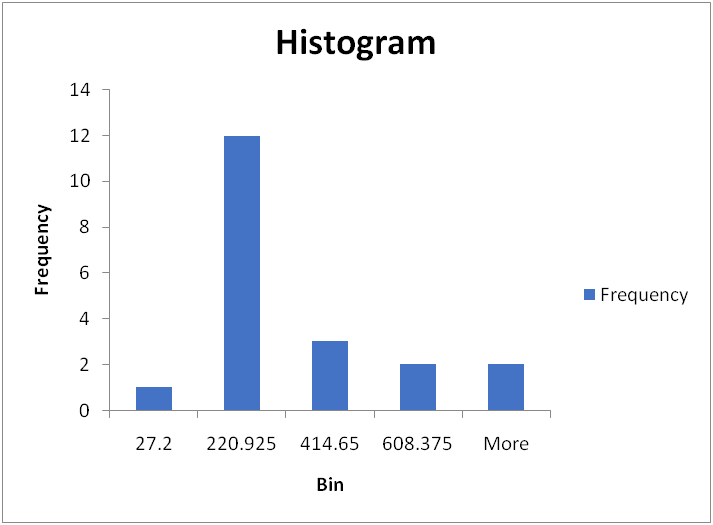
- In Excel, generate a histogram for the Sales variable. Reference characteristics of the histogram as you discuss the shape of the variable distribution.
- Can the empirical rule be applied to the Sales variable? Justify your response referencing details contained in the course materials for this week.
- Calculate the Z-score for the Salesvalue for row 14 in the spreadsheet (162.9). Report the formula you used. Is the Sales value for row 14 above or below the variable’s mean? Justify your response referencing the Z-score results that you calculated.
Assignment solution
2.
| Variables | Level of measurement |
| comp. million | Ratio |
| sales | Ratio |
| no. employees | Ordinal |
| cap. investment | Ratio |
| manufacturing | Nominal |
| Statistics | comp. million | sales | no. employees | cap. investment | manufacturing |
| Mean | 335.85 | 207.02 | 1321.75 | 61.025 | 0.5 |
| Standard Error | 23.96854024 | 51.788985 | 329.0443489 | 17.11125649 | 0.114707867 |
| Median | 307 | 106.15 | 674.5 | 26.45 | 0.5 |
| Mode | xx | xx | xx | xx | 1 |
| Standard Deviation | 107.1905706 | 231.60738 | 1471.531064 | 76.52386539 | 0.512989176 |
| Sample Variance | 11489.81842 | 53641.98 | 2165403.671 | 5855.901974 | 0.263157895 |
| Kurtosis | -0.541795383 | 1.8435322 | 1.724095663 | 2.845672912 | -2.235294118 |
| Skewness | 0.763031425 | 1.6113973 | 1.587621283 | 1.820972612 | 0 |
| Range | 352 | 774.9 | 4740 | 274.6 | 1 |
| IQR | 166.75 | 241.2 | 1486.25 | 68.7 | 1 |
| Minimum | 212 | 27.2 | 156 | 3.8 | 0 |
| Maximum | 564 | 802.1 | 4896 | 278.4 | 1 |
| Sum | 6717 | 4140.4 | 26435 | 1220.5 | 10 |
| Count | 20 | 20 | 20 | 20 | 20 |
In the above table, the mean and median for all the variables were presented. On average, the company had a sale of 207.02 with a median of 106.15, capital investment with an average of 61.025 and a median of 26.45, and 1322 employees were employed by the company on average with a median of 675 employees. As evident in the table, the means of all the variables except capital investment are greater than their respective medians. On the measure of variability, a standard deviation that shows how varied observations are from the mean is reported in the above table, also, Range and Interquartile range were presented in the same table. Variability is lowest in capital investment (SD = 76.5) followed by comp.million (SD = 107.17), then sales (SD = 231.6) and no. employees (SD = 1471.53). The interquartile range which is the difference between the 75th percentile and 25th percentile gives a spread of observations. From the table, it is observed that there is much spread of observation in the number of employees followed by sales, comp. million and then capital investment. Skewness is simply a measure of asymmetry and normal distribution has a skewness of zero. From the table, all the variables have skewness greater than 0 which implies that the variables are not normally distributed. The shape is equally not symmetrical. Hence, the variables are right-skewed. On the kurtosis of the distribution, which measures the peakedness of the distribution. A normal distribution has a kurtosis of 3 or excess kurtosis of 0, a kurtosis of less than -1 is too flat while a kurtosis of more than is too peaked. from the table, it is observed that comp. million is too flat (Platykurtic) while the sales, capital investment, and the number of employees is too peaked (leptokurtic).
4.
Mean is the better measure of central tendency for comp. million, sales, no. of employees, and capital investment due to their scales of measurement. However, manufacturing which is measured at a nominal level is best described using the median as its measure of central tendency.
5.
| Statistics | capital investment |
| Min. | 3.8 |
| Q1 | 10.95 |
| Q2 | 26.45 |
| Q3 | 79.65 |
| Max. | 278.4 |
| IQR | 68.7 |
IQR=Q_3-Q_1
IQR=68.7
This tells us that the middle 50% of values in capital investment have a spread of 68.7
6.
From the box plot presented above, two observations are identified as outliers which are 222.2 and 278.4, looking at the five summary statistics, the distribution is not symmetrical in shape.
7.
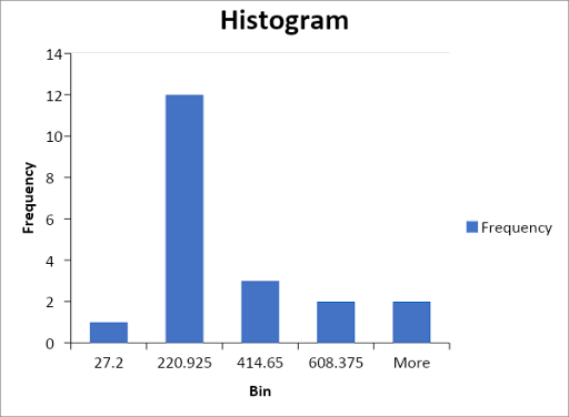
Since most of the values are clustered on the right side of the histogram with a single peak, the histogram is unimodal in shape and right-skewed.
8.
The empirical rule cannot be applied to the sales variable since the variable is not symmetrical in shape which implies nonnormality. The empirical rule applies to variables that are symmetrical in nature.
9.
Z= (x-μ)/σ
For samples,
the Z-score for the Sales value for row 14 in the spreadsheet (162.9) is
The value of the Z-score implies that the sales value of 162.9 is a 0.19 standard deviation below the mean