Problem Description
This Data Analysis Homework focuses on creating data visualizations using SAS Studio. You will work with the "Covid19DataCDC.xlsx" data file for the first two questions and some SASHELP data files for the remaining questions. The goal is to generate insightful graphics and provide analyses for each visualization.
Solution
PROC PRINT DATA = SASHELP.DATA (OBS = 10);
RUN; where DATA on the right side of = should be replaced with specific data used in each question code.
Question 1: This first question is based on “Covid19DataCDC.xlsx” that you used in Data Visualization Project 5. Go to the CODE tab of the file that appears when you import the Excel data file into SAS Studio and run the CODE. This action will show IMPORT within the temporary library WORK in your session of SAS Studio. In the following code, use WORK.IMPORT in the DATA statement is equivalent to using the “Covid19DataCDC.xlsx” dataset. Copy the following SAS code, paste it into the SAS Program file in your SAS Studio, and run it. You will see a needle plot displaying new COVID-19 cases (new_case) for California (CA) over the period of 403 days. Below the code on this Word file, you should display this graph [5 points]. Below this graph, write a paragraph to summarize the trend of new COVID-19 cases in CA for the entire period of submission date [5 points].
PROC SGPLOT DATA = WORK.IMPORT (WHERE = (state = 'CA'));
TITLE 'Trend of New COVID-19 Cases in California';
NEEDLE x = submission_date y = new_case / MARKERS
MARKERATTRS = (SYMBOL = circlefilled SIZE = 5px);
YAXIS GRID LABEL = 'New COVID-19 Cases';
XAXIS GRID LABEL = 'Submission Date';
RUN;
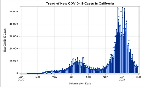
From the plotted graph, we can see the trend of the new cases of Covid-19 from January 2020 to March 2021. We can clearly note low Cases experienced in 2020 with a first rise in cases between July and September and later a reduction in the cases. However, in the wake of December 2020 to January 2021, High number of Covid cases reported. The highest number of cases ever reported. In the subsequent months, we can see a steady reduction in the number of newly reported cases in California state.
Question 2: The following code (after you fill in the blank) can be used to produce a comparative needle plot, which will help facilitate a comparison between California (CA) and New York City (NYC). Your task is to copy the code, paste it into the SAS Program file, complete the code by filling in the blank (…), and run it. Below the code on this Word file, you should display this graph [5 points]. Below this graph, first, write the code that you used to fill in the blank and then write a paragraph to compare the trend of new COVID-19 cases between CA and NYC [5 points].
PROC SGPLOT DATA=WORK.IMPORT (where=(state=('NYC') & ('CA')));
TITLE 'Trend of New COVID-19 Cases between California and New York City';
NEEDLE x=submission_date y=new_case / GROUP=state MARKERS
MARKERATTRS=(SYMBOL=circlefilled SIZE=5px);
YAXIS GRID LABEL='New COVID-19 Cases';
XAXIS GRID LABEL='Submission Date';
RUN;
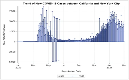
From the plot diagram above, we can notice two faces of the spike in the number of newly reported cases in both California and New York City. Between the months of April 2020 to May 2020 and a steady increase between November 2020 all the way to January 2021. Between July 2020 to October 2020, we can see a steady small number of newly reported cases. In the subsequent months between February to March 2021, there is a reduction in the number of newly reported cases however, it is still high compared to the lowest period of between July 2020 to October 2020.
Question 3: The following code can be used to produce a Scatterplot Matrix, which shows scatterplots in the upper and lower triangles of the matrix and histograms in the diagonal of the matrix. Copy the code, paste it into the SAS Program, and run it. You will see a scatterplot matrix in the RESULTS tab. Look at the histograms in the diagonal and three pairwise scatterplots in the lower triangle to answer the second part of this question. Below the code on this Word file, you should display this scatterplot matrix [5 points]. Below this matrix, write a paragraph to summarize the pairwise relationships of Diastolic, Systolic (measurements of Blood Pressure), and Cholesterol with each other. Also, explain whether each of the variables is normally distributed [5 points].
PROC SGSCATTER DATA = SASHELP.HEART;
TITLE 'Scatterplot Matrix for Heart Data';
MATRIX Diastolic Systolic Cholesterol / DIAGONAL = (HISTOGRAM NORMAL);
RUN;
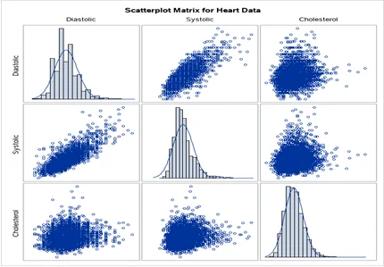
The link between high blood pressure and high cholesterol goes in both directions. It shows the bivariate relationships between Blood Pressure and cholesterol and depicts that when the blood pressure increases so does the cholesterol. On the scatterplot matrix, we also have the histogram plot showing the distribution of the variables in the data set. The distribution of diastolic is fairly normal with a high peak while the distribution for systolic is positively skewed and highly peaked and Cholesterol is also highly peaked and positively skewed. There is a positive correlation between cholesterol diastolic, and systolic. This means that as cholesterol levels increase, the higher the risk of blood pressure.
Question 4: The following code (after you fill in the blank) can be used to produce a Scatterplot Matrix for the three variables Diastolic, Systolic, and Cholesterol for Overweight Male patients from the SASHELP.HEART dataset. Your task is to copy the code, paste it into the SAS Program file, complete the code by filling in the blank (…), and run it. Below the code on this Word file, you should display this scatterplot matrix [5 points]. Below this matrix, first write the code that you used to fill the blank and then write a paragraph to summarize the pairwise relationships of Diastolic, Systolic, and Cholesterol with each other. Also, explain whether each of the variables is normally distributed [5 points].
PROC SGSCATTER DATA = SASHELP.HEART (where=(sex='Male'));
TITLE 'Scatterplot Matrix for Overweight Male Patients from Heart Data';
MATRIX Diastolic Systolic Cholesterol / DIAGONAL = (HISTOGRAM NORMAL);
RUN;
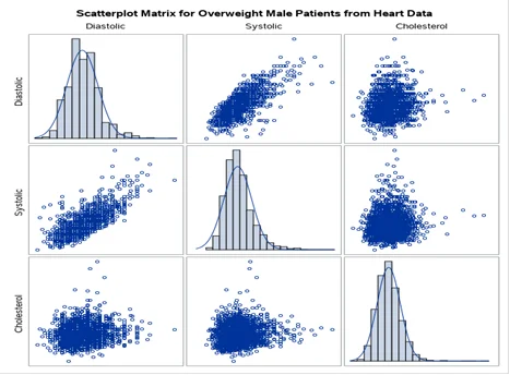
For male patients in this data set, the histogram plots show a highly peaked distribution that is fairly normal for both diastolic, systolic and cholesterol levels. For male patients, the link between high blood pressure and high cholesterol goes in both directions. The relationship is positive from the scatterplot between cholesterol and systolic and cholesterol and diastolic. This shows that for male patients, consumption of higher levels of cholesterol is highly associated with high blood pressure.
Question 5: The following code can be used to produce a Heatmap plot of Weight vs. Height of Male patients from HEART (Framingham Heart Study) data. Copy the code, paste it into the SAS Program, and run it. Below the code on this Word file, you should display this graph [5 points]. Below this graph, write a paragraph to summarize the relationship of the two variables, Weight and Height, for this subgroup. In your summary, mention how this heatmap is different from the scatterplot that could be used to show the relationship between the two variables. [5 points].
PROC SGPLOT DATA = SASHELP.HEART (WHERE = (sex = 'Male'));
TITLE 'Heatmap for Weight vs. Height for Male Patients from Heart Data';
HEATMAP y = Weight x = Height;
RUN;
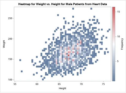
From the heatmap above, we can see a plot of the Height and weight of the male patients in this data set. Clearly, we can note that a high number of males in this dataset weighed between 150 and 200 and were of a height between 65 to 70. Heart disease is always related to huge weights and heights and from the data set, we can note that with larger weights, and larger heights, the more prone a male is to succumbing to heart disease.
Question 6: The following code can be used to produce a Dot Plot of mean Systolic blood pressure of Female patients whose status was Alive from SASHELP.HEART data. Copy the following code, paste it into the SAS Program, and run it. Below the code on this Word file, you should display this graph [5 points]. Below this graph, write a paragraph to summarize the data displayed on this graph, especially by mentioning the differences in the mean Systolic blood pressure by Smoking [5 points].
PROC SGPLOT DATA = SASHELP.HEART (WHERE = (Status = 'Alive' & sex = 'Female'));
TITLE 'Average Systolic BP by Smoking for Alive Female Patients from Heart Data';
DOT smoking / RESPONSE = Systolic STAT = mean LIMITS = both;
RUN;
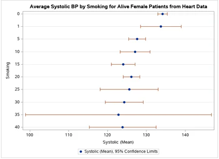
From the dataset, the average systolic blood pressure of females who were alive ranges from 120 to 130 for smokers. For those who did not smoke frequently, they have normal blood pressure levels. High-frequency smokers had either high blood pressure levels or low blood pressure levels. This shows that smoking is a determinant of the blood pressure levels of females gauging from this data set. The differences in blood pressure levels from various smoking frequency shows how smoking is a significant contributor to heart disease in general.