Problem Description:
In this Data Analysis homework, we delve into election data from Naples, Italy. The dataset provides information on the number of valid votes for various political leaders in different municipalities within the Naples district. The dataset contains voting numbers for six political leaders: Berlusconi, Bersani, Grillo, Monti, Ingroia, and others. With a total of 450,372 voting observations, our objective is to conduct a Correspondence Analysis (CA) to explore the association between these two categorical variables, the municipalities' voting behavior and the political leaders. The primary aim of this analysis is to gain a deeper understanding of the voting patterns across Naples, Italy.
Solution:
Results and Interpretations
Test of independence between the rows and the columns:
| Chi-square (Observed value) | 11925.220 |
|---|---|
| Chi-square (Critical value) | 61.656 |
| DF | 45 |
| p-value | <0.0001 |
| alpha | 0.050 |
Smallest P value <0.0001 the chi-square is significant, and the 2 variables are not independent
Total inertia = 0.026
Interpretation: Total inertia is the Chi-squared divided by the total number of observations (n) which provides an indicator of the total information to explain.
The total inertia also known as total weighted Variance explained by the five components is calculated to be 0.026 as highlighted above.
Eigenvalues and percentages of inertia:
| F1 | F2 | F3 | F4 | F5 | |
|---|---|---|---|---|---|
| Eigenvalue | 0.017 | 0.008 | 0.002 | 0.000 | 0.000 |
| Inertia % | 63.852 | 29.301 | 5.834 | 0.674 | 0.340 |
| Cumulative % | 63.852 | 93.153 | 98.986 | 99.660 | 100.000 |
First, it appears that, with a single dimension, 63.85% of the inertia can be explained, that is, the relative frequency values that can be reconstructed from a single dimension can reproduce 63.85% of the total Chi-square value for this two-way table; two dimensions allow us to explain 93.15 %.
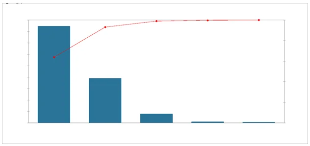
Interpretation: Through analyzing the percentages of inertia, we can determine that 93.15% of the observations are determined by the first two factors within the dataset. As such, the analysis of voting behavior across the municipalities will be on the basis of F1 and F2.
According to the graph above, only dimensions 1 and 2 should be used in the solution. The dimension 3 explains only 0,2% of the total inertia which is below the average.
Profiles (rows):
| Berlusconi | Bersani | Grillo | Monti | Ingroia | Others | Sum | |
|---|---|---|---|---|---|---|---|
| M01 | 0.325 | 0.282 | 0.194 | 0.152 | 0.022 | 0.025 | 1.000 |
| M02 | 0.313 | 0.303 | 0.238 | 0.083 | 0.039 | 0.023 | 1.000 |
| M03 | 0.310 | 0.296 | 0.253 | 0.081 | 0.038 | 0.021 | 1.000 |
| M04 | 0.351 | 0.267 | 0.252 | 0.068 | 0.034 | 0.028 | 1.000 |
| M05 | 0.224 | 0.368 | 0.232 | 0.115 | 0.041 | 0.020 | 1.000 |
| M06 | 0.292 | 0.339 | 0.246 | 0.065 | 0.030 | 0.028 | 1.000 |
| M07 | 0.406 | 0.219 | 0.241 | 0.079 | 0.028 | 0.026 | 1.000 |
| M08 | 0.337 | 0.254 | 0.259 | 0.081 | 0.041 | 0.028 | 1.000 |
| M09 | 0.329 | 0.259 | 0.270 | 0.079 | 0.043 | 0.022 | 1.000 |
| M10 | 0.228 | 0.343 | 0.272 | 0.088 | 0.048 | 0.021 | 1.000 |
| Mean | 0.312 | 0.293 | 0.246 | 0.089 | 0.036 | 0.024 | 1.000 |
Interpretation: The above table indicates the percentage of the population who vote for each political leader within each municipality.These are the values the will be plotted on the row oriented plot.CA investigates the differences between each individual row profile and the average row profile
From the table above we can observe that 31.2 % of the population in Naples voted for Berlusconi vs. 29.3% who voted for Bersani, followed by Grillo at 24.6%. Even though Berlusconi received a majority of votes, we can observe varied positions of different municipalities based on their political inclinations. For example, a larger proportion of Municipality 5 voted for Bersani (36.8%) vs. Berlusconi (22.4%). On the other hand, a large proportion of the population in Municipality 1 voted for Berlusconi (32.5%) vs. Bersani (28.2%). Further investigation is required to understand each municipality’s political inclination and their voting behavior according to the political leaders.
In M01 and M07 , M05 people vote in different way
Principal coordinates (rows):
| F1 | F2 | F3 | F4 | F5 | |
|---|---|---|---|---|---|
| M01 | -0.005 | 0.248 | 0.004 | 0.011 | -0.005 |
| M02 | -0.012 | -0.015 | 0.012 | -0.021 | 0.019 |
| M03 | -0.020 | -0.031 | -0.002 | -0.015 | -0.010 |
| M04 | -0.124 | -0.042 | 0.024 | 0.008 | 0.005 |
| M05 | 0.208 | 0.036 | -0.002 | -0.010 | 0.004 |
| M06 | 0.032 | -0.072 | 0.090 | 0.010 | -0.006 |
| M07 | -0.243 | 0.032 | 0.008 | -0.010 | -0.005 |
| M08 | -0.106 | -0.023 | -0.035 | 0.022 | 0.017 |
| M09 | -0.087 | -0.047 | -0.056 | -0.006 | -0.010 |
| M10 | 0.153 | -0.078 | -0.040 | 0.015 | -0.005 |
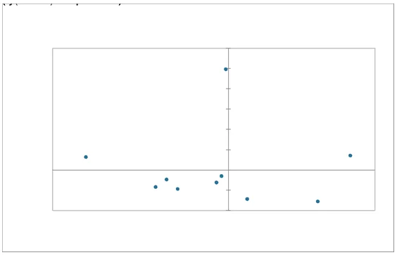
Interpretation: the above symmetric row plot provides a distribution of municipality voting based on Factor 1 and Factor 2 which explains 93.15% of the variability and relationship. The row plot graph shows that municipality 7, 5 and 1 distributions are farthest from the mean, indicating that those municipalities have the strongest political inclinations. From the graph we can interpret that M7 and M5 are opposite with respect to the voting behavior and which political party they lean towards. we can see that if two points are close to each other that means they share a similar profile , like M02 and M03.
Principal coordinates (rows):
| F1 | F2 | F3 | F4 | F5 | |
|---|---|---|---|---|---|
| M01 | -0.005 | 0.248 | 0.004 | 0.011 | -0.005 |
| M02 | -0.012 | -0.015 | 0.012 | -0.021 | 0.019 |
| M03 | -0.020 | -0.031 | -0.002 | -0.015 | -0.010 |
| M04 | -0.124 | -0.042 | 0.024 | 0.008 | 0.005 |
| M05 | 0.208 | 0.036 | -0.002 | -0.010 | 0.004 |
| M06 | 0.032 | -0.072 | 0.090 | 0.010 | -0.006 |
| M07 | -0.243 | 0.032 | 0.008 | -0.010 | -0.005 |
| M08 | -0.106 | -0.023 | -0.035 | 0.022 | 0.017 |
| M09 | -0.087 | -0.047 | -0.056 | -0.006 | -0.010 |
| M10 | 0.153 | -0.078 | -0.040 | 0.015 | -0.005 |
In this correspondence analysis, 5 factors were considered in the row analysis which 10 municipalities across the political leaders. From the results presenter, M01, M05 and M10 shows greater variability among all the municipalities. The sum of the modulus of the first first factors is more than that of the of the last three. Hence, the first two factors F1 and F2 are sufficient and highly significant in explaining explaining the variability and relationships among the municipalities.
Contributions (rows):
| Weight (relative) | F1 | F2 | F3 | F4 | F5 | |
|---|---|---|---|---|---|---|
| M01 | 0.093 | 0.000 | 0.740 | 0.001 | 0.060 | 0.021 |
| M02 | 0.087 | 0.001 | 0.003 | 0.009 | 0.214 | 0.345 |
| M03 | 0.099 | 0.002 | 0.012 | 0.000 | 0.120 | 0.113 |
| M04 | 0.085 | 0.078 | 0.019 | 0.032 | 0.029 | 0.020 |
| M05 | 0.149 | 0.383 | 0.025 | 0.000 | 0.080 | 0.027 |
| M06 | 0.106 | 0.006 | 0.070 | 0.563 | 0.059 | 0.041 |
| M07 | 0.079 | 0.275 | 0.011 | 0.003 | 0.047 | 0.022 |
| M08 | 0.085 | 0.056 | 0.006 | 0.067 | 0.234 | 0.266 |
| M09 | 0.106 | 0.047 | 0.030 | 0.211 | 0.025 | 0.108 |
| M10 | 0.110 | 0.152 | 0.085 | 0.113 | 0.134 | 0.037 |
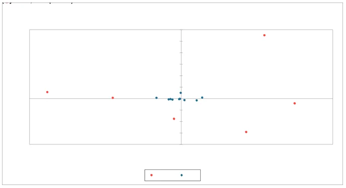
Interpretation: the above asymmetric row plot provides the distribution of both the municipalities and the political leaders based on the two main factors F1 and F2. This graph helps visually understanding the relationship between municipalities and the political leaders. For example, we can understand from the graph that a large proportion of the population in municipalities M05, 06 and 10, vote for Bersani whereas municipalities M07, 08, 04, and 09 vote for Berlusconi with respect to the mean because the points are attracted by Berlusconi with respect to the mean . M10 the proportional voted for Ingroia Is greater with respect to the other.
Each point is the body center of the red points using weight which reflect how much the municipality voted for the candidate with respect to the other municipality .
Squared Cosines (rows):
| F1 | F2 | F3 | F4 | F5 | Sum of F1 and F2 | |
|---|---|---|---|---|---|---|
| M01 | 0.000 | 0.997 | 0.000 | 0.002 | 0.000 | 0.998 |
| M02 | 0.105 | 0.172 | 0.117 | 0.335 | 0.272 | 0.276 |
| M03 | 0.241 | 0.567 | 0.003 | 0.128 | 0.061 | 0.808 |
| M04 | 0.865 | 0.098 | 0.033 | 0.003 | 0.001 | 0.963 |
| M05 | 0.969 | 0.028 | 0.000 | 0.002 | 0.000 | 0.997 |
| M06 | 0.071 | 0.354 | 0.566 | 0.007 | 0.002 | 0.425 |
| M07 | 0.980 | 0.017 | 0.001 | 0.002 | 0.000 | 0.997 |
| M08 | 0.814 | 0.040 | 0.089 | 0.036 | 0.021 | 0.854 |
| M09 | 0.581 | 0.170 | 0.239 | 0.003 | 0.007 | 0.751 |
| M10 | 0.748 | 0.193 | 0.051 | 0.007 | 0.001 | 0.941 |
Interpretation: the squared cosines are used to indicate the level of significance of the observations within the data set. We take the sum of the squared cosines of F1 and F2 to determine the level of significance against each municipality and validate. Given the sum of F1 and F2 for all municipalities is above 0.05 we can conclude that factor 1 and 2 show a high level of significance to explain the voting behavior of all municipalities.
The result of the analysis shows that the contingency table has been successfully represented in low dimension space using correspondence analysis. The two factors 1 and 2 are sufficient to retain 93,15% of the total inertia (variation) contained in the data. However, not all the points are equally well displayed in the two dimensions. If a row item is well represented by two dimensions, the sum of the cos2 is close to one like M01,M07,M05. For some of the row items, more than 2 dimensions are required to perfectly represent the data like M02.
Profiles (columns)
| Berlusconi | Bersani | Grillo | Monti | Ingroia | Others | Mean | |
|---|---|---|---|---|---|---|---|
| M01 | 0.100 | 0.088 | 0.074 | 0.157 | 0.055 | 0.099 | 0.095 |
| M02 | 0.090 | 0.088 | 0.085 | 0.080 | 0.093 | 0.085 | 0.087 |
| M03 | 0.101 | 0.098 | 0.102 | 0.089 | 0.101 | 0.089 | 0.097 |
| M04 | 0.099 | 0.076 | 0.088 | 0.064 | 0.078 | 0.100 | 0.084 |
| M05 | 0.111 | 0.184 | 0.141 | 0.189 | 0.166 | 0.122 | 0.152 |
| M06 | 0.102 | 0.120 | 0.106 | 0.077 | 0.087 | 0.123 | 0.103 |
| M07 | 0.105 | 0.057 | 0.077 | 0.069 | 0.061 | 0.087 | 0.076 |
| M08 | 0.094 | 0.072 | 0.090 | 0.076 | 0.094 | 0.101 | 0.088 |
| M09 | 0.115 | 0.091 | 0.116 | 0.092 | 0.122 | 0.096 | 0.105 |
| M10 | 0.083 | 0.126 | 0.122 | 0.107 | 0.142 | 0.098 | 0.113 |
| Sum | 1.000 | 1.000 | 1.000 | 1.000 | 1.000 | 1.000 | 1.000 |
We can see in the graph the distribution of the votes in differents municipalitie , we see that berlusconi and bersani are opposite with respect these profiles , first we can notice that they are different from the mean because they are far from the origin, they behave in opposite ways because they may have municipalities more habitant where the votes are higher and the other less people vote with respect these profile to these column Bersusconi and bersani behave different in opposite way with respect to the mean and others .we can see in the table that the M01 vote by 10% to Berlusconi whereas for Bersani only 8.8%.
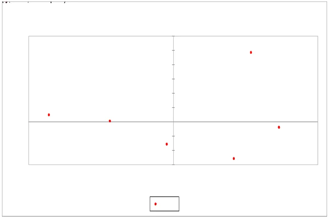
Principal coordinates (columns):
| F1 | F2 | F3 | F4 | F5 | |
|---|---|---|---|---|---|
| Berlusconi | -0.172 | 0.025 | 0.013 | -0.008 | 0.002 |
| Bersani | 0.146 | -0.019 | 0.037 | -0.005 | 0.001 |
| Grillo | -0.009 | -0.078 | -0.032 | 0.009 | -0.010 |
| Monti | 0.107 | 0.243 | -0.049 | 0.005 | -0.002 |
| Ingroia | 0.084 | -0.129 | -0.120 | -0.017 | 0.034 |
| Others | -0.088 | 0.003 | 0.064 | 0.071 | 0.029 |
Presented in the table above are five principal coordinates for the political leaders across the ten municipalities with different magnitudes. The most significant coordinates are the first two which are F1 and F2 as highlighted in the table. This implies that the conclusion that will be drawn when all the coordinates are been evaluated is almost the same as that of the first two coordinates. In all the coordinates, there are equal positive and negative values except F5.
Going by the mean, all political leaders received the most valid votes from M05, Monti received the highest valid votes among the political leaders following by Bersani and then Ingroia. The remaining political leaders had lesser votes compared to the three leaders mentioned.
Contributions (columns):
| Weight (relative) | F1 | F2 | F3 | F4 | F5 | |
|---|---|---|---|---|---|---|
| Berlusconi | 0.303 | 0.533 | 0.024 | 0.035 | 0.096 | 0.009 |
| Bersani | 0.300 | 0.378 | 0.014 | 0.261 | 0.044 | 0.002 |
| Grillo | 0.246 | 0.001 | 0.193 | 0.160 | 0.115 | 0.285 |
| Monti | 0.091 | 0.062 | 0.690 | 0.139 | 0.015 | 0.004 |
| Ingroia | 0.037 | 0.015 | 0.079 | 0.342 | 0.058 | 0.470 |
| Others | 0.024 | 0.011 | 0.000 | 0.063 | 0.672 | 0.230 |
In the above table, the relative weight is presented for all the political leaders. On the average, Berlusconi had more valid votes across municipalities with 30.3% contributions followed by Bersani with 30% contributions and Grillo with 24.6% contributions. The remaining political leaders contribute only 15% collectively.
Conclusion
Overall, the data analysis above provided insightful information to municipalities voting behaviors across the different candidates. We can see from the above-mentioned results and interpretation the following key conclusions:
- Berlusconi was the lead contender with respect to number of votes, where 31.2% of the population of Naples voted for him, followed by Bersani in second position who gathered 29.3% of the votes in Naples.
- The political leaders Berlusconi, Bersani, and Grillo made up 85.1% of the total votes.
- Berlusconi and Bersani are positioned on opposite sides of the political party, in which Berlusconi is the right wing and Bersani is left wing.
- Municipality 7 had the largest proportion of their population voting for Berlusconi, while Municipality 5 had the largest proportion of voters for Bersani.
- Voters for Grillo in Municipality 1 were particularly low due to divergence in political inclination and thinking.
- The other candidates within the elections tended to be more aligned with the right-wing, potentially additional votes away from Berlusconi.
- Although Ingroia only succeeded in taking 3.6% of the total votes in Naples, his party affiliation was more left-wing, thus potentially taking away votes from Bersani.
- Municipalities 2 and 3 were closest to the mean, indicating that their population was even split with respect to votes between the different political leaders.