Instructions
Research Question:
The consequences of marijuana criminalization in the United States
Time period: 2010-2018
Operationalized Hypothesis- With the legalization of marijuana, it would eliminate the unfair race and community-targeted enforcement of marijuana criminal laws. Thus with the legalization of marijuana in states increasing, a African American arrest charge decreases.
Unit analysis- marijuana possession arrest
● Independent Variable: Marijuana legalization
● Dependent Variable: # of arrest made
● Control Variables: Sex, Age, and Race
● Sample Size: 100,000
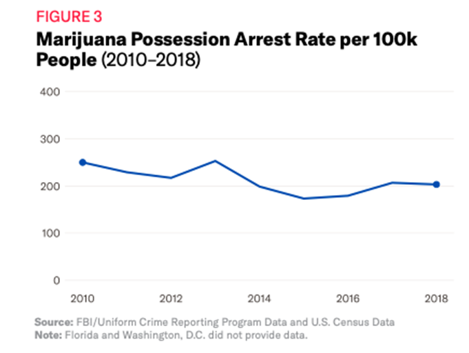
The national marijuana possession arrest rate in 2018 was 203.88 per 100,000. State arrest rates ranged from 707.34 arrests per 100,000, in South Dakota, to 4.52 arrests per 100,000 people, in Massachusetts (see Appendix, Table A for data for all states). Not only did South Dakota have the highest arrest rate in 2018 (see Figure 5), it also had the greatest growth, with a 176% increase in marijuana possession arrests from 2010. Although nationally there was a decline in marijuana possession arrests, arrest rates actually increased in 17 states (see Table 2).
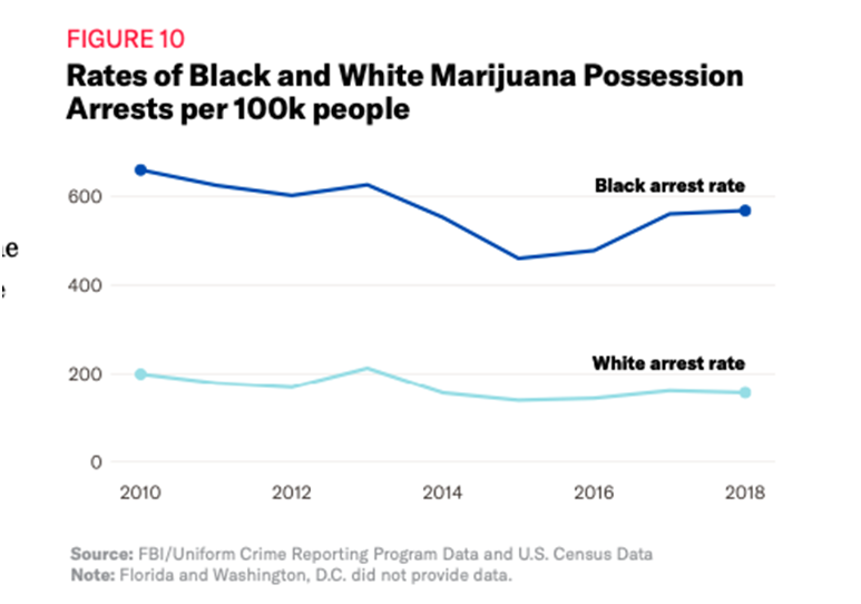
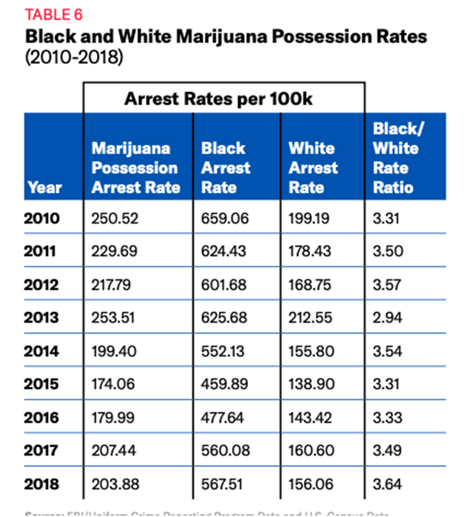
Rates of Black and White Marijuana Possession Arrests per 100k people
1.
Descriptive Statistics
–
Provide a “Descriptive Statistics Table” of variables showing
mean, standard error, ..., sum, and count
–
Provide a paragraph of explanation about descriptive
2.
Scatterplot: Visualization and Bivariate Analysis
–
Create a scatterplot using the dependent variable and
independent variable
Provide a scatterplot with a trend line, a regression
equation, and R-squared
–
Provide an interpretation of the scatterplot. In other words,
provide an explanation about the effect of the independent
variable on the dependent variable in terms of...
Existence, magnitude, and direction of the effect
3.
Inference Statistics: Multivariate Analysis
–
Provide a multivariate regression result table
–
Write a regression equation based on the regression result
–
Provide explanations about the result
What is your level of significance (i.e. alpha)? “0.05 (5%)”
What is your explanatory power of regression equation as
a whole
–
Interpret both R-sq. and Adjusted R-sq.
Is your overall regression model statistically significant?
–
Test the overall model significance by comparing the P-value of F (i.e., Significant F) and alpha
Provide explanations about a result(s) (cont.)
Interpret y-intercept
Interpret the regression coefficient on the independent
variable. Also, explain its statistical significance by
comparing a P-value and alpha
**
–
Test (accept or reject) your alternative hypotheses (i.e.
your hypothesis = your tentative answer for your
research question)
Interpret regression coefficients on each control variable.
Also, explain their statistical significance by comparing P-
values and alpha
4.
Data
(Appendix I)
–
Complete the data spreadsheet (i.e. your raw data table)
Write appropriate
variable labels
of each variable
Table need to show
units
of each variable
Code
/enter data properly, especially a dummy variable
(0 or 1)
–
Provide
final “Data Set Table”
Copy an Excel spreadsheet of raw data and paste it on
MS-Word your assignment
5.
Statistical Diagnosis
(Appendix II)
–
If you use a cross-sectional data, then check:
Multicollinearity
using “Variance Influence Factor (VIF)”
–
If you use a time-series data or panel data, then check:
Multicollinearity
and
Autocorrelation
using “Durbin-Watson statistic”
–
Provide each diagnostics processes and outputs and interpret
those results
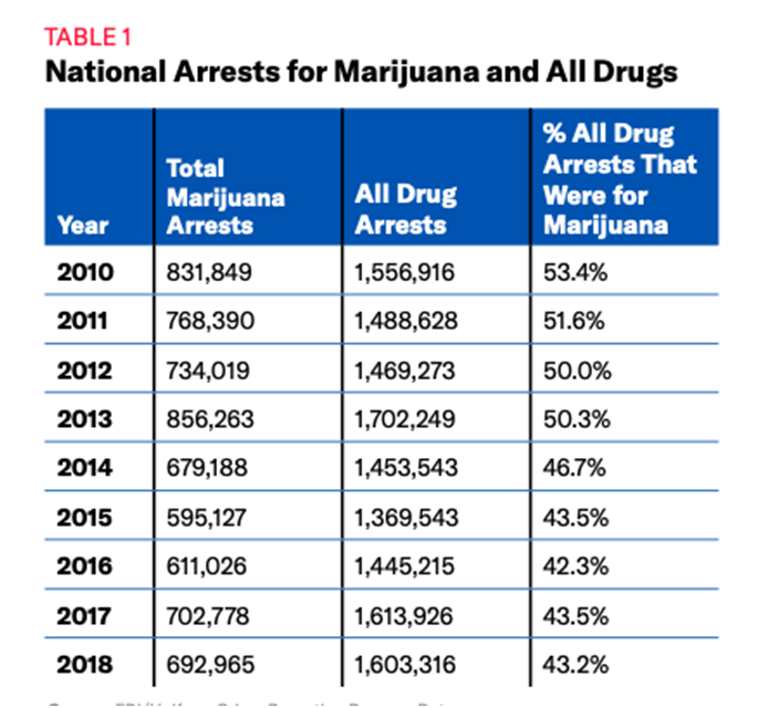
So to clarify, we are looking at data between 2010-2018 of marijuana arrest rates and marijuana arrest rates between blacks and whites. Looking at a sample size of 100,000
Assignment Solution
1. Descriptive Statistics Table
| Count | Sum | Range | Min. | Max. | Mean | Variance | Skewness | Kurtosis | |
|---|---|---|---|---|---|---|---|---|---|
| # Arrests | 49 | 12358 | 740 | 13 | 753 | 252.21 | 34130.399 | 0.871 | 0.568 |
The dataset used for the analysis has 49 observations with 13 as the least number of marijuana arrests and 753 as the highest. The data for the Marijuana arrests case is positively skewed and this means that its mean value of 252.21 is greater than the median of the data point. A standard deviation of 184.744 indicates a greater spread in the observations, that is, most of the observations are spread within 92 standard deviations on each side of the mean. The data has a leptokurtic distribution because the distribution has heavier tails.
2. Scatterplot: Visualization and Bivariate Analysis
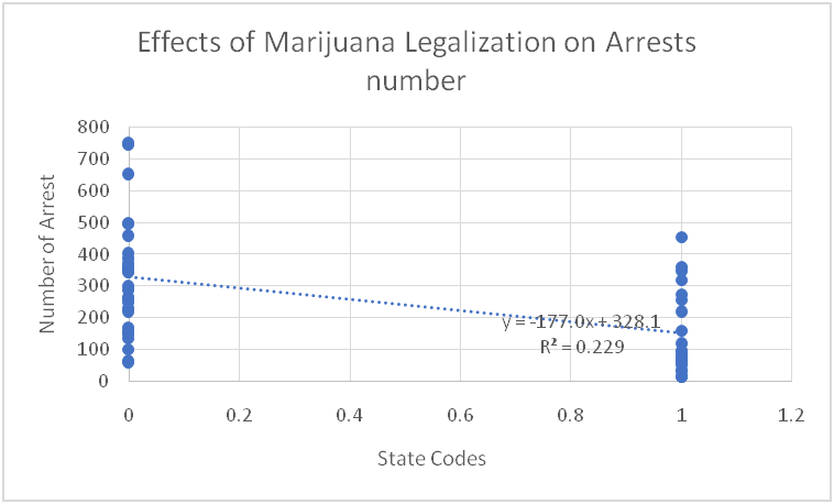
The shape of the scatterplot between the number of arrests across 49 states in the United States of America indicates a non-linear negative relationship between the dependent variable (Number of arrests) and the independent variable (Marijuana legalization). The scatterplot also portrays the regression equation, trendline, and R-squared. In summary, Marijuana legalization has a non-linear negative impact on a number of arrests and cases related to marijuana.
3. Inferential Statistics
| Regression Statistics | |
|---|---|
| Multiple R | 0.479266109 |
| R Square | 0.229696003 |
| Adjusted R Square | 0.213306557 |
| Standard Error | 163.8601872 |
| Observations | 49 |
| ANOVA | ||||||
|---|---|---|---|---|---|---|
| df | SS | MS | F | Significance F | ||
| Regression | 1 | 376301.6 | 376301.6 | 14.01487 | 0.000494 | |
| Residual | 47 | 1261958 | 26850.16 | |||
| Total | 48 | 1638259 |
| Coefficients | S. Error | t Stat | P-value | |
|---|---|---|---|---|
| Intercept | 328.1032 | 30.96666 | 10.59537 | 4.79E-14 |
| Code | -177.083 | 47.30236 | -3.74364 | 0.000494 |
| State | Code | Arrests |
|---|---|---|
| Alabama | 0 | 63.06 |
| Alaska | 1 | 57.72 |
| Arizona | 0 | 220.01 |
| Arkansas | 0 | 358.79 |
| California | 1 | 13.79 |
| Colorado | 1 | 91 |
| Connecticut | 1 | 64.77 |
| Delaware | 1 | 118.9 |
| Georgia | 0 | 499.68 |
| Hawai‘i | 0 | 59.18 |
| Idaho | 0 | 351.37 |
| Illinois | 1 | 76.17 |
| Indiana | 0 | 286.73 |
| Iowa | 0 | 147.8 |
| Kansas | 0 | 99.8 |
| Kentucky | 0 | 170.07 |
| Louisiana | 0 | 459.82 |
| Maine | 1 | 61.64 |
| Maryland | 1 | 317.86 |
| Massachusetts | 1 | 13.13 |
| Michigan | 0 | 156.98 |
| Minnesota | 1 | 158.83 |
| Mississippi | 1 | 348.68 |
| Missouri | 1 | 359.93 |
| Montana | 0 | 135.19 |
| Nebraska | 1 | 453.58 |
| Nevada | 1 | 95.6 |
| New Hampshire | 1 | 219.2 |
| New Jersey | 0 | 404.67 |
| New Mexico | 0 | 249.93 |
| New York | 0 | 300.26 |
| North Carolina | 1 | 256.4 |
| North Dakota | 0 | 354.04 |
| Ohio | 1 | 272.79 |
| Oklahoma | 0 | 229.69 |
| Oregon | 1 | 77 |
| Pennsylvania | 0 | 264.87 |
| Rhode Island | 1 | 49.93 |
| South Carolina | 0 | 753.11 |
| South Dakota | 0 | 746.68 |
| Tennessee | 0 | 387.44 |
| Texas | 0 | 259.08 |
| Utah | 0 | 372.71 |
| Vermont | 1 | 33.56 |
| Virginia | 0 | 344.02 |
| Washington | 1 | 30.94 |
| West Virginia | 0 | 496.32 |
| Wisconsin | 0 | 360.59 |
| Wyoming | 0 | 655 |