Time series presentation and analysis
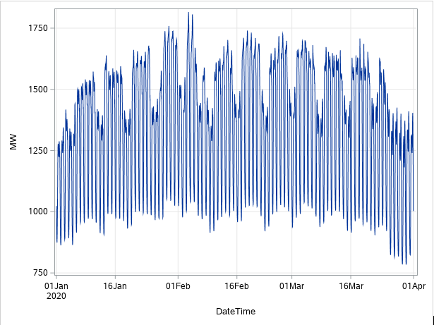
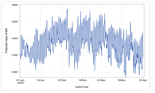
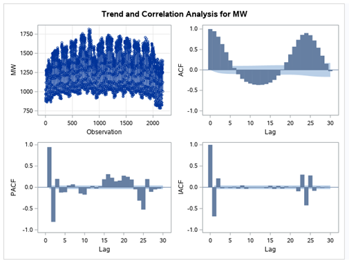
The time series plot is presented below. The plot shows there is no trend in electricity consumption but there is evidence of seasonality in the plot. Moreover, the mean returns to a constant trend which suggests stationarity of the series.
Questions
1. Data Organization and Preliminary Assessment
(a) Import the data.
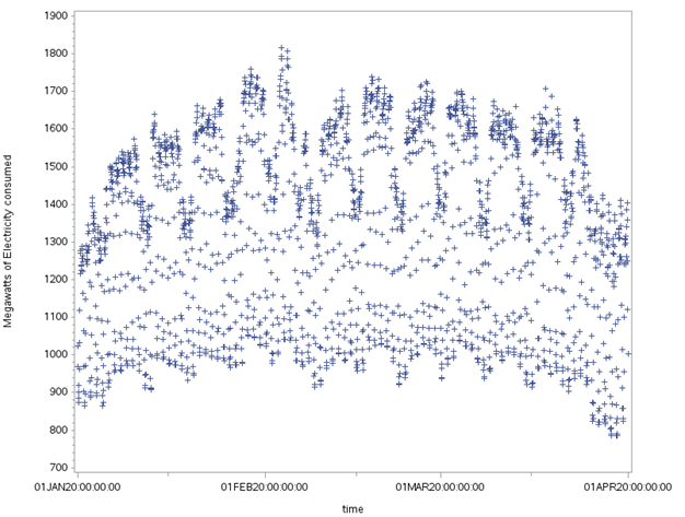
(b) Make an appropriate plot and discuss the main features of the hourly electricity demand data.
2. Time Series Regression and Exponential Smoothing
(a) Fit the time series regression model for the hourly electricity demand data, use the model to forecast the demand for seven days, and discuss the results.
(b) Find an appropriate exponential smoothing method for the hourly electricity demand data, make the forecasts for seven days, and discuss the results.
3. ARIMA and ARIMAX
(a) Find an appropriate ARIMA model for the hourly electricity demand data, make the forecasts for seven days, and discuss the results.
(b) Find an appropriate ARIMA model for the hourly electricity demand data with the temperature and the wind speed as the explanatory variables, and discuss the results.
4. Out-of-Sample Forecasts
(a) Hold the last seven days of data as the test set and use the rest as the training set.
(b) Evaluate the forecast accuracy from the models and methods in Questions 2 and 3, and choose the best forecasting model/method.
Solution:
The plot shows there is no trend in electricity consumption even though evidence of seasonality in the plot. Additionally, the mean returns to a constant trend which is a clear indication of a stationary series.
Solution 2
Time series regression model
The time series regression model is
MW=α_0+α_1 temperature_t+α_2 windspeed_t+ε_t
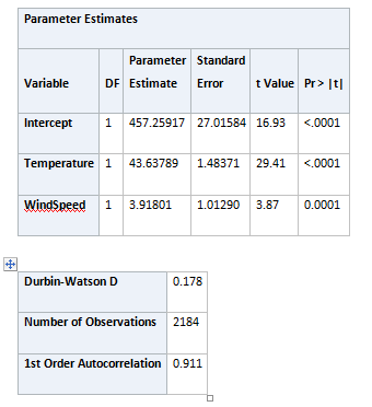
The result of the model is presented below. Both independent variables are significant. They explain 35.34% of the variation in the dependent variables. the DW stat is close to 2 which shows there is no autocorrelation.
The plot of predicted values and forecast is presented below. we see that the forecast shows a similar pattern as the actual values.
B
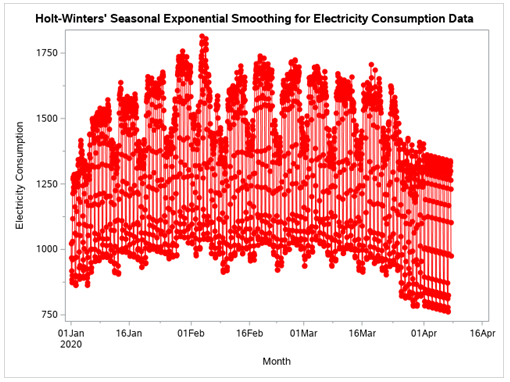
Since there is seasonality in the dataset, we used the additive Holt winters model. The estimated coefficient for the parameters is shown in the table. We see that the alpha used for the model is 0.999 while the beta is 0.001 and the gamma is 0.999.
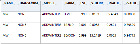
The plot of original values and forecast is presented below
Solution 3
Establishing ARIMA Model
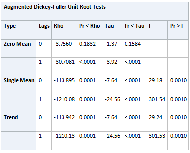
We first determine the stationary status of megawatts of electricity consumed using the ADF test. The result is presented below. From the result, we see that p<.005 which means we can reject the null hypothesis that the variable is not stationary at levels. Thus the variable is stationary.
Next, we identify the AR and MA orders. The ACF is used to identify the MA order and seasonal order while the PACF is used to identify the AR order. Looking at the plot, we see that one or two AR terms, one MA term, and one seasonal AR and MA term are appropriate. Thus, we estimated three models SARIMA (1,0,1) (0,0,1), SARIMA (2,0,1) (0,0,1),and SARIMA (1,0,1) (1,0,1). We see that SARIMA (2,0,1) (0,0,1) is better as it has the lowest AIC value.
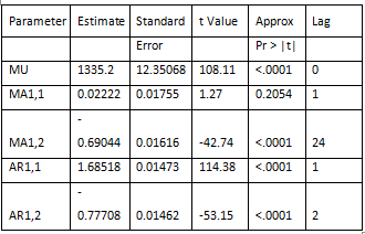
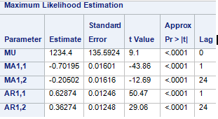
Thus, we estimate it and use it for forecasts. The estimated value is presented below
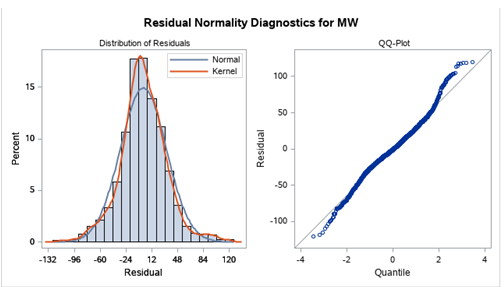
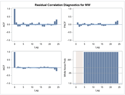
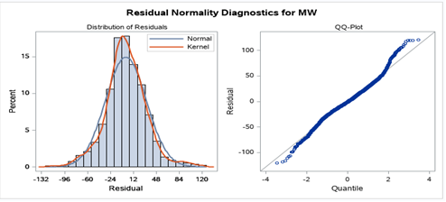
The plot of the residuals shown below indicates that the model satisfies the no autocorrelation of residuals and normality assumptions.

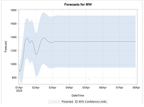
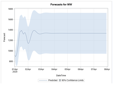
The plot of the forecast for the next seven days is presented below. We see that the forecasted value becomes constant after some periods.
B
To forecast for ARIMAX, we need to identify the stationarity, AR, and MA term for the independent variables which are temperature and wind speed. First, both variables are stationary. For temperature, the model we used after a careful look at the ACF and PACF is ARIMA (2,0,2)(1,0,0) while for windspeed ARIMA (0,0,2) is better.
Then using SARIMA (2,0,1) (0,0,1) for MW as identified from the cross-correlation and correlation plots. The residual diagnostic plot below shows assumptions regarding normality and autocorrelation of residuals were met.
The coefficient estimate of the model is shown in the table below. The result shows that all the AR terms and MA terms are significant.
The forecast for the next seven days is presented below. the result shows that the forecasted value becomes a constant at some point.
Solution 4
ARIMA Sample Forecast
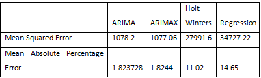
The result of the accuracy is presented below. The ARIMA model has the lowest Mean Absolute Percentage Error while ARIMAX has the lowest Mean Squared Error. Thus, if we go by Mean Squared Error, ARIMAX is the best. On the other hand, if we decide by Mean Absolute Percentage Error, ARIMA is the best