Problem Description:
The Time Series Analysis using R homework requires the analysis and cleaning of a time series dataset containing at least two predictor variables and one response variable (yt). The goal is to determine a model that best fits the data. The provided dataset can be downloaded from Kaggle:
Solution
Select a time series dataset which contains at least two predictor variables and one response variable (yt). We need to analyze and clean the data to ascertain a model which best fits the data.
##https://www.kaggle.com/datasets/yasserh/wine-quality-dataset/download?datasetVersionNumber=1
##the dataset can be downloaded and saved.
1. Exploratory Data Analysis
- First check for completeness and consistency of the data (if there are NAs or missing observations, replace with the value of the previous observation; make a note of this)
- Provide descriptive analyses of your variables. This should include the five-number summary, histograms with fitted distribution, correlation plots (or heatmap). All figures must include comments.
mydata<-read.csv("C:UsersUserOneDriveDesktop>winequality-red.csv",header =T,sep = ",")
mydata1<-(mydata[,1:3])
summary(mydata1)
fixed.acidity volatile.acidity citric.acid
Min. : 4.60 Min. :0.1200 Min. :0.000
1st Qu.: 7.10 1st Qu.:0.3900 1st Qu.:0.090
Median : 7.90 Median :0.5200 Median :0.260
Mean : 8.32 Mean :0.5278 Mean :0.271
3rd Qu.: 9.20 3rd Qu.:0.6400 3rd Qu.:0.420
Max. :15.90 Max. :1.5800 Max. :1.000
## Plotting a histogram
fixed.acidity <- mydata$fixed.acidity
hist(fixed.acidity)
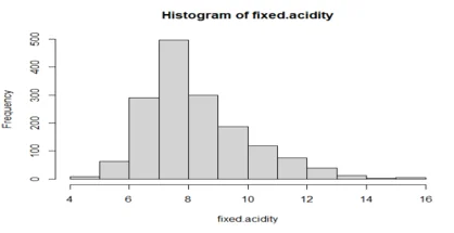
## the data is normally distributed as show above
# plotting corr heatmap
# Load and install heatmaply package
install.packages("heatmaply")
library(heatmaply)
heatmaply_cor(x = cor(mydata1), xlab = "Features",
ylab = "Features", k_col = 2, k_row = 2)
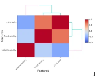
## Colinearity between different features can be observed
2. Data pre-processing
(a) With tsdisplay or ggtsdisplay, for each variable, use its time series plot, ACF and PACF to comment on its stationarity (you can also decompose the time series). To supplement this, use the appropriate Dickey-Fuller (unit root) test, to determine whether or not it is stationary.
# Importing library
install.packages("tseries")
library(tseries)
## for first variable (volatile.acidity)
mydata2<-(mydata[,1:2])
mydata2
mydata2<-as.data.frame(mydata1)
wine.ts1<-ts(mydata2[,2], frequency=4)
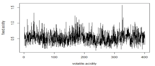
#par(mfrow=c(3,1), mar=c(4,4,4,4)) ### Figure 4.5
plot(wine.ts1, type="l", xlab="volatile.acidity",ylab="fixed.acidity")
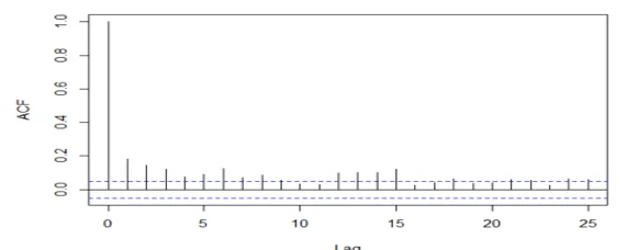
acf(mydata2[,2], 25, xlab="Lag", ylab="ACF", main="")
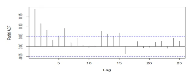
acf(mydata2[,2], 25, type="partial", xlab="Lag",ylab="Partial ACF", main="")
## for second variable (citric.acid)
mydata3<-(mydata[,3])
mydata3
mydata3<-as.data.frame(mydata1)
wine.ts2<-ts(mydata3[,2], frequency=4)
#par(mfrow=c(3,1), mar=c(4,4,4,4)) ### Figure 4.5
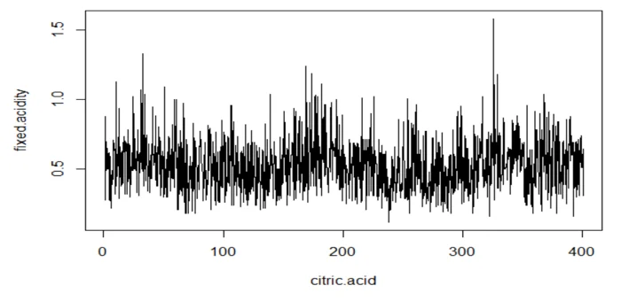
plot(wine.ts2, type="l", xlab="citric.acid",ylab="fixed.acidity")
acf(mydata3[,2], 25, xlab="Lag", ylab="ACF", main="")
# Conduct the augmented Dickey-Fuller test
data1=mydata$volatile.acidity
data2=mydata$citric.acid
adf.test(data1)
Augmented Dickey-Fuller Test
data: data2
Dickey-Fuller = -8.62, Lag order = 11, p-value = 0.01
alternative hypothesis: stationary
The test statistic and p-value come out to be equal to -8.62 and 0.01 respectively.
Since the p-value is less than 0.05 we would reject the null hypothesis. It implies that the time series is stationary.
adf.test(data2)
Augmented Dickey-Fuller Test
data: data2
Dickey-Fuller = -7.2507, Lag order = 11, p-value = 0.01
alternative hypothesis: stationary
## The test statistic and p-value come out to be equal to -7.2507and 0.01 respectively.
Since the p-value is less than than 0.05, we would reject the null hypothesis. It implies that the time series is stationary.
(b) If it is not stationary, determine the level of differencing to make our series stationary. We can use the ndiffs function which performs a unit-root test to determine this. After this, difference your data to ascertain a stationary time series. Re-do part c) for your differenced time series and comment on the time series plot, ACF and PACF. Recall that the time series models we’ve observed rely on stationarity.
#Difference the data
dwine1<-diff(mydata2[,2], lag=4)
#par(mfrow=c(3,1), mar=c(4,4,4,4)) ### Figure 4.6
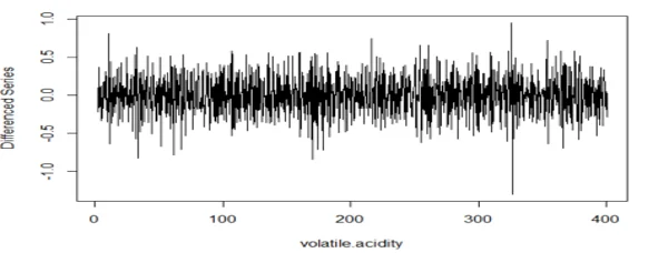
plot(diff(wine.ts1, lag=4), type="l", xlab="volatile.acidity",ylab="Differenced Series")
acf(dwine1, 25, xlab="Lag", ylab="ACF", main="")
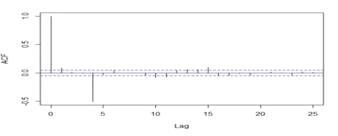
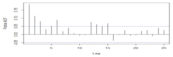
acf(dwine1, 25, type="partial", xlab="Lag",ylab="Partial ACF", main="")
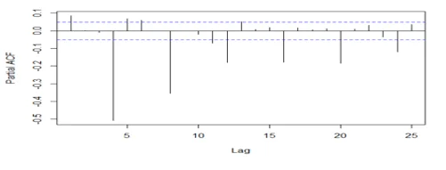
## The series is stationary since the ACF cuts off at lag one and the PACF attenuates.
3. Feature Generation, Model Testing and Forecasting.
(a) Fit an AR(p) model to the data (using part (a), AIC or some built in R function)
#Fitting the model
dwine1.aic<-matrix(0,5,5)
for (i in 0:4) for (j in 0:4) {
dwine1.fit<-arima(dwine1, order=c(i,0,j))
dwine1.aic[i+1,j+1]<-dwine1.fit$aic
}
dwine1.fit<-arima(dwine1, order=c(3,0,4))
dwine1.fit
Call:
arima(x = dwine1, order = c(3, 0, 4))
Coefficients:
ar1 ar2 ar3 ma1 ma2 ma3 ma4
0.1165 0.0627 0.0377 0.0202 0.0216 0.0253 -0.9679
s.e. 0.0264 0.0262 0.0264 0.0085 0.0082 0.0085 0.0081
intercept
0e+00
s.e. 6e-04
install.packages("dLagM")
library(dLagM)
data(mydata)
model.ardlDlm1 = ardlDlm(formula =fixed.acidity ~ volatile.acidity + citric.acid,
data = data.frame(mydata) , p = 2 , q = 1 )
summary(model.ardlDlm1)
Time series regression with "ts" data:
Start = 3, End = 1599
Call:
dynlm(formula = as.formula(model.text), data = data)
Residuals:
Min 1Q Median 3Q Max
-5.6897 -0.7233 -0.0334 0.7063 6.6500
Coefficients:
Estimate Std. Error t value Pr(>|t|)
(Intercept) 3.72772 0.24723 15.078 < 2e-16 ***
volatile.acidity.t 1.44002 0.20717 6.951 5.28e-12 ***
volatile.acidity.1 -0.19413 0.21183 -0.916 0.3596
volatile.acidity.2 0.11671 0.20695 0.564 0.5729
citric.acid.t 6.43283 0.19860 32.392 < 2e-16 ***
citric.acid.1 -1.61361 0.25607 -6.301 3.81e-10 ***
citric.acid.2 0.45340 0.19801 2.290 0.0222 *
fixed.acidity.1 0.29360 0.02403 12.216 < 2e-16 ***
---
Signif. codes: 0 ‘***’ 0.001 ‘**’ 0.01 ‘*’ 0.05 ‘.’ 0.1 ‘ ’ 1
Residual standard error: 1.21 on 1589 degrees of freedom
Multiple R-squared: 0.5196, Adjusted R-squared: 0.5175
F-statistic: 245.5 on 7 and 1589 DF, p-value: < 2.2e-16
4. Provide a brief summary of your findings and state which model performs better.
## adjusted R2. is 0.5175 which means that at least half of the response variable is explained by the predictor variables.
This model has equally distributed residuals around zero. The errors of this model are within a small bandwidth.
This fitted model therefore performs better than the first two models.
5. Suggest any improvements which could’ve been made to the model based on your findings, and what was learnt in class.
From the finding we can see that an increase in volatile. acidity increase the fixed. acidity positively also Increase in citric.acid increase the fixed.acidity
Thus, both should be controlled at an average level.