Statistical management report
The solution below is a statistical-based report on the prices of gas in the rich neighborhoods against the richer neighborhoods. The report found that the prices of gas were 5% higher in the poorer neighborhoods.
Task
Step 1: Present a brief introduction to your Management Report. That is, describe the purpose, assumptions, and objectives of your Report as well as a brief description or outline of the data collection and analysis. The purpose of this section is to tell your client the scope of your report.
Step 2: State the complete hypothesis (as presented in Section 9.1 of your textbook). That is, you should present both a null (H0) and an alternate hypothesis (Ha). Be sure to provide the hypothesis in the correct notation (H0 & Ha) as well as in a narrative format.
Step 3: Describe the data analysis (i.e., hypothesis test) process. This DOES NOT include a step-by-step process of Excel steps. Instead, it DOES include a narrative of the comparison process required to test the hypothesis described in Step 2, above. In addition, you must include at least 2 graphical displays and 3 numerical measures of the data and describe/explain their relevance with respect to this project (in Step 6 below).
Step 4: Test your hypothesis. Using inferential statistics, test your hypothesis using a t-test (Two-Sample Assuming Equal Variances). You must show the statistical analysis results (mean, t-critical, t-stat, significance level, etc.) relative to a normal distribution (see example posted in the project folder).
Step 5: State your conclusion (i.e., results of your hypothesis test) and whether you accept or reject the Null hypothesis, and how you reached this conclusion. It might be helpful to utilize the normal distribution provided in Step 4 to explain your conclusion.
Step 6: Provide a recommendation to EDA with respect to the gasoline prices and what implications this may have for EDA. This section should also describe the graphical displays and numerical measures associated with the data and explain/justify why the specific recommendation is being made.
Solution:
Step 1: Introduction
The city of Hamilton Economic Development Agency (EDA) is a think-tank, advocate, and consulting company that assists the city and businesses in attracting new business and developing existing businesses to the
community. The apparent economic differences between the city's richer and poorer neighborhoods have long been a source of concern for the EDA. That is, the richer areas are thriving owing to new businesses, reduced prices, and increased construction, whilst the poorer neighborhoods are failing due to decaying infrastructure, rising costs, and a general population exodus. The objective of this project is to determine if the gas prices in poorer neighborhoods are higher than the wealthier neighborhoods. The data for this project is collected in Hamilton city between the poor and wealthier neighborhoods. The data measures the retail gasoline price in the poor and wealthier neighborhoods between January 2019 to December 2019. The data is collected on a weekly basis.
Step 2: Hypothesis
In this project, the null and alternative hypothesis is given below:
Null hypothesis: the gas prices in the poorer neighborhoods and wealthier neighborhoods are the same.
Alternative hypothesis: the gas prices in the poorer neighborhoods are higher than the wealthier neighborhoods.
H_0:μ_1=μ_2
H_a:μ_1>μ_2
Where μ_1 = mean of gas prices in the poor neighborhood
Where μ_2 = mean of gas prices in the wealthier neighborhood
Step 3: Data Analysis
In other to achieve the goal of this project, exploratory data analysis will be carried out on the dataset, followed by inferential statistical analysis. The most appropriate statistical test for this research is the independent sample t-test. Independent sample t-test is an inferential statistical test that determines whether there is a statistically significant difference between the means in two unrelated groups (Poorer and wealthier neighborhoods).
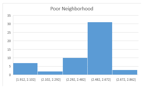
The Histogram chart above shows that the gasoline price in the poorer neighborhood has a left-skewed (negatively skewed) distribution. That’s because there is a long tail in the negative direction on the number line. The mean is also to the left of the peak. This implies that more gasoline prices in the poorer neighborhood fall below the mean.
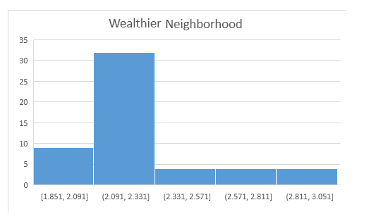
The Histogram chart above shows that the gasoline price in the wealthier neighborhood has a right-skewed (positively skewed) distribution. That’s because there is a long tail in the positive direction on the number line. The mean is also to the right of the peak. This implies that more gasoline prices in the wealthier neighborhood fall above the mean.
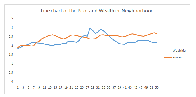
The line chart above shows the relationship of gasoline prices between the poorer and wealthier neighborhoods.
Descriptive statistics
| N | Mean | Median | Mode | Standard Deviation | |
Wealthier Neighborhood | 53 | 2.279 | 2.199 | 2.167 | 0.259 |
Poorer Neighborhood | 53 | 2.455 | 2.527 | 2.571 | 0.207 |
The descriptive statistics show that the average price of gasoline in the wealthier neighborhood is 2.279 (SD = 0.259) and the average price of gasoline in the poorer neighborhood is 2.455 (SD = 0.207).
Step 4: Hypothesis testing
The mean and standard deviation of gasoline price in the wealthier neighborhood is (2.279, 0.259) respectively and (2.455, 0.207) for the wealthier neighborhood respectively.
There was a significant effect for Hamilton city neighborhood,t(stat) = -3.867, t(104) = -3.867, t(critical) = 1.660, p < .05, with the poorer neighborhood receiving higher gasoline price than the wealthier neighborhood.
Step 5: Conclusion
The test is statistically significant because there is enough evidence to support the researcher's claim at a 5% level of significance. We, therefore, conclude that the gas prices in the poorer neighborhoods are higher than the wealthier neighborhoods.
Step 6: Recommendation
Based on the result carried out to determine if the gas prices in the poorer neighborhoods are higher than the wealthier neighborhoods, we found out that the test is statistically significant with a 5% level of significance.
The mean gas price of the poorer neighborhood (2.455) is higher than the higher neighborhood (2.279), which is due to business risk (assumed by the business owner), lower supply (not as many stores), and lower mobility (residents don’t travel very far or very frequently), etc. The histogram graph also shows that more of the gasoline price falls above the mean of the poorer neighborhood compare to the wealthier neighborhood.
Since the hypothesis is significant, therefore, EDA can put forward an economic development plan that would make great strides to improve and rebuild the poorer neighborhoods. This may help to ease congestion on the city's northern borders, as a result bringing jobs and riches to the city's poorest neighborhoods (which are strategically located close to the downtown business district).