Problem Description:
This Statistical Analysis Homework involves various datasets, "Psych_Data.xlsx," to draw meaningful conclusions from the data. The dataset contains information related to psychological aspects. Below are the main analyses conducted in the homework:
Solution
***Assume alpha = .05 for all questions on this homework***
1. (a) What type of hypothesis test will you run?
Since the dependent variable (anxiety scores) used is a scale variable and the independent variable is a categorical variable with two categories (Yes/No), an independent samples t-test is used to run the analysis.
(b) State the Ho and Ha.
Let μ1= mean anxiety score of subjects who have insurance
Let μ2= mean anxiety score of subjects with no insurance
H0:μ1=μ2
Ha:μ1≠μ2
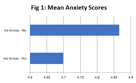
(c) Include descriptive statistics (mean, standard deviation, sample size) AND an appropriate graphical display that allows you to visually compare the Anxiety Scores for the two Medical Insurance groups.
The descriptive statistics presented in Table 1 for anxiety scores based on two medical Insurance groups show that the average anxiety score for subjects without medical insurance (M=4.87) is higher than the average anxiety score for subjects with medical insurance (M=4.70). The same is also presented in Figure 1. Another measure of central tendency, the median, is also larger for subjects without medical insurance (Median=5.00) than the subjects with medical insurance (M=4.65). The spread of the data as measured by standard deviation is, however, higher for subjects with medical insurance (SD=1.05) than subjects without medical insurance (SD=0.99). Another measure of spread, the range (which is a difference between maximum and minimum) is also higher for subjects with medical insurance (3.5) than subjects without medical insurance (3.4). Inter-quartile range, another measure of dispersion (difference between third and first quartile) is lower for subjects with medical insurance (1.5) than subjects without medical insurance (1.65).
Table 1: Descriptive Statistics for Anxiety Score for subjects with medical insurance and without medical insurance
| Statistics |
Ins Group - Yes |
Ins Group - No |
Overall |
|
|---|---|---|---|---|
| Sample Size |
66 |
64 |
130 |
|
| Mean |
4.6985 |
4.8656 |
4.7808 |
|
| St Dev |
1.0520 |
0.9922 |
1.0 |
|
| Minimum |
3.0000 |
3.0000 |
3.0 |
|
| Q1 |
3.8000 |
4.0500 |
3.83 |
|
| Median |
4.6500 |
5.0000 |
4.95 |
|
| Q3 |
5.7000 |
5.7000 |
5.70 |
|
| Maximum |
6.5000 |
6.4000 |
6.5 |
d) Give the test statistic, p-value, and decision from your test results.
Table 2: Independent samples t-test results
| test statistic: |
0.9322 |
|---|---|
| p-value: |
0.353 |
| Decision: |
Fail to reject Ho |
(e) Write a full conclusion (in context) for the results of this test in a way that can be understood by a non-statistical person. This answer will be at least 100 words or more.
As seen earlier, the descriptive statistics presented in table 1 for anxiety scores based on two medical Insurance groups show that the average anxiety score for subjects without medical insurance (M=4.87, SD=0.99) is higher than the average anxiety score for subjects with medical insurance (M=4.70, SD=1.05). The independent samples t-test conducted to compare the mean anxiety scores based on the two medical Insurance groups namely with and without medical insurance concluded that there exists no statistically significant difference in the mean anxiety scores on the basis of whether the subjects have medical insurance or not (t = 0.93, p =0.353).
2. (a) What type of hypothesis test will you run?
Since the dependent variable (Suicide Risk levels) used is a scale variable and the independent variable (ses levels) is a categorical variable with three categories (1, 2 and 3), one-way ANOVA is used to run the analysis.
(b) State the Ho and Ha.
Let μ1= mean suicide risk level for SES Level 1
Let μ2= mean suicide risk level for SES Level 2
Let μ3= mean suicide risk level for SES Level 3
H0:μ1=μ2=μ3
Ha: At least one mean suicide risk level is significantly different
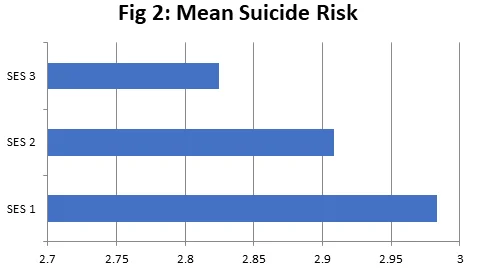
(c) The descriptive statistics presented in table 3 for suicide risk levels based on SES groups show that the average suicide risk levels for subjects in SES1 group (M=2.98) are higher than the average suicide risk levels for subjects in SES2 group (M=2.91) which is higher than the average suicide risk levels for subjects in SES3 group (M=2.825). The same is also presented in Figure 2. Another measure of central tendency, the median, is also larger for subjects SES1 group (Median=3.15) than the subjects in the SES2 group (M=2.85) which is larger than for subjects in the SES3 group (Median = 2.7).
The spread of the data as measured by standard deviation is, however, highest for subjects in the SES3 group (SD=0.874) and lowest for subjects in the SES2 group (SD=0.81). Another measure of spread, range (which is a difference between maximum and minimum), however, is highest for subjects in the SES3 group (3.1) and lowest for subjects in the SES2 group (2.7). Inter-quartile range, another measure of dispersion (difference between the third and first quartile) is also largest for the SES3 group (2.625) and lowest for the SES2 group (1.45).
Table 3: Descriptive Statistics for Suicidal Risk Levels
| Statistics |
SES 1 |
SES 2 |
SES 3 |
Overall |
|---|---|---|---|---|
| |
|
|
|
|
| Sample Size |
48 |
46 |
36 |
130 |
| Mean |
2.9833 |
2.9087 |
2.8250 |
2.9131 |
| St Dev |
0.8618 |
0.8107 |
0.8739 |
0.84325 |
| Minimum |
1.4000 |
1.5000 |
1.1000 |
1.1 |
| Q1 |
2.2000 |
2.2000 |
2.1000 |
2.20 |
| Median |
3.1500 |
2.8500 |
2.7000 |
2.85 |
| Q3 |
3.7250 |
3.6500 |
3.7250 |
3.70 |
| Maximum |
4.3000 |
4.2000 |
4.2000 |
4.3 |
(d) Give the test statistic, p-value, and decision from your test results. Would a post-hoc be necessary – why or why not?
Table 4: One-way ANOVA results
| test statistic: |
0.359 |
|---|---|
| p-value: |
0.698 |
| Decision: |
Fail to reject Ho |
| Post-Hoc |
Not Needed |
(e) Write a full conclusion (in context) for the results of this test in a way that can be understood by a non-statistical person. This answer will be at least 100 words or more.
As seen earlier, the descriptive statistics presented in table 3 for suicide risk levels based on SES groups show that the average suicide risk levels for subjects in the SES1 group (M=2.98) are higher than the average suicide risk levels for subjects in the SES2 group (M=2.91) which is higher than the average suicide risk levels for subjects in SES3 group (M=2.825). One-way ANOVA conducted to compare the mean suicide risk levels based on the three SES groups namely 1, 2, and 3 concluded that there exists no statistically significant difference in the mean suicide risk levels on the basis of different SES groups (F = 0.36, p =0.698).
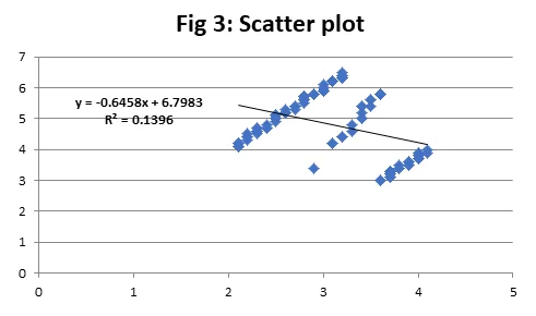
3. a) Create a scatterplot to display this relationship. Use the graph to describe the relationship between the two variables in terms of shape and direction.
The scatter plot presented in Figure 3 between depression level and anxiety score shows a downward sloping trendline which means there exists a negative relation between the two variables i.e. higher the depression level, the lower the anxiety score, and vice versa. However, the slope of the trendline is not very steep which means that the relationship between the two variables is not very strong.
(a) Generate the appropriate regression analysis in Excel and paste your results here.
Table 5: Regression Results from Excel
| SUMMARY OUTPUT |
||||||
|---|---|---|---|---|---|---|
| Regression Statistics |
||||||
| Multiple R |
0.373627 |
|||||
| R Square |
0.139597 |
|||||
| Adjusted R Square |
0.132875 |
|||||
| Standard Error |
0.952118 |
|||||
| Observations |
130 |
|||||
| ANOVA |
||||||
| |
df |
SS |
MS |
F |
Significance F |
|
| Regression |
1 |
18.82629 |
18.82629 |
20.76746 |
1.2E-05 |
|
| Residual |
128 |
116.0356 |
0.906528 |
|||
| Total |
129 |
134.8619 |
|
|
|
|
| |
Coefficients |
Standard Error |
t Stat |
P-value |
Lower 95% |
Upper 95% |
| Intercept |
6.798253 |
0.450516 |
15.08993 |
3.42E-30 |
5.906831 |
7.689676 |
| dep_scale |
-0.64583 |
0.141719 |
-4.55713 |
1.2E-05 |
-0.92625 |
-0.36542 |
(c) What is the value of the correlation coefficient? Is there a positive or negative association? Is the association weak, moderate, or strong?
The value of the correlation coefficient is -0.374. This suggests that there exists a negative association. Since the value of the correlation coefficient is neither close to 0 nor to 1, and this value is mid-way between 0 and 1, the association is moderate.
(d) Based on the Excel output above, is there convincing evidence of a significant linear relationship between Anxiety Score and Depression Level (yes or no)? Explain how you know.
The p-value of the F-test is close to zero. Since this is a simple regression, we can conclude that there exists convincing evidence of a significant linear relationship between Anxiety Score and Depression Level (yes or no)
(e) Using your Excel output above, write the prediction equation (should be in the form y ̂=b_0+b_1 x). Then, using your equation, predict the Anxiety Score for a subject with a Depression Level of 3.4 (round your answer to two decimal places). SHOW WORK for your calculation.
The prediction equation is y ̂=6.7983-0.6458x
The predicted value for a subject with a Depression level of 3.4
= 6.7983- 0.6458*3.4
= 6.9311- 2.1957
= 4.6026
4. (a) What type of hypothesis test will you run?
Since the dependent variable (mental health status) used is a scale variable and the independent variable (pre and post therapy) is a categorical variable with two categories (before/after) and the subjects being compared are the same, paired samples t-test is used to run the analysis.
(b) State the Ho and Ha.
Let μd = mean difference in scores
(post_ther - pre_ther)
H0:μd = 0
Ha:μd > 0
(b) Give the test statistic, p-value, and decision from your test results.
Table 6: Paired samples t-test results
| test statistic: |
-33.54797 |
|---|---|
| p-value: |
1 |
| Decision: |
Fail to Reject Ho |
(d) Write a full conclusion (in context) for the results of this test in a way that can be understood by a non-statistical person. This answer will be at least 100 words or more.
The paired samples t-test is conducted to test if there has been an improvement in one’s mental health status using a short-term integrated therapy method where the mental health scores are measured before and after the therapy. The results from the paired samples t-test show that the p-value of the test is close to 1. At a 5% alpha level, since this value is larger than 0.05, we cannot reject the null hypothesis and conclude that there exists no statistically significant difference in one’s mental health status using a short-term integrated therapy method. Moreover, the test statistic (post-pre) is negative which means that there is not an improvement in one’s mental health status and the average difference in post and pre-mental health status is negative.
5. From the Psych_Data.xlsx dataset, use the ethnicity and therapy_pref variables to determine whether there is evidence of a significant association between ethnicity and preferred therapy method (individual, group, mixed).
(a) What type of hypothesis test will you run?
Since the two variables (ethnicity and preferred therapy) used are categorical variables, chi-square test for independence is used to run the analysis.
(b) State the Ho and Ha.
H0: Therapy preference is not associated with Ethnicity
Ha: Therapy preference is associated with Ethnicity
(c) Include an appropriate graphical display that allows you to visually assess the association between ethnicity and therapy preference. Copy/paste the graph here. Comment on any association that appears to be present.
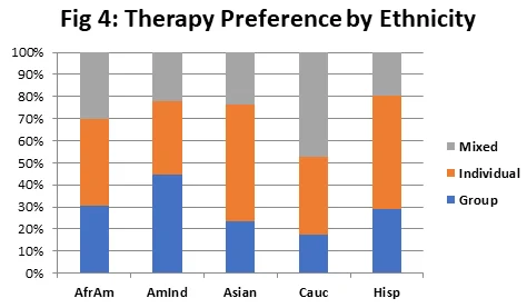
Figure 4 shows that between 15 to 30% of the subjects have “group” therapy preference for all ethnicities except “AmInd” where this % is quite high. Individual preference is higher for Asians and Hispanics, followed by other three ethnicities. Caucasians have largest mixed preference. The overall trend is not very clear.
(c) Give the test statistic, p-value, and decision from your test results.
Table 6: Chi-square test for independence results
| test statistic: |
9.788 |
|---|---|
| df |
8 |
| p-value |
0.280 |
| Decision |
Do not Reject null |
(e) Write a full conclusion (in context) for the results of this test in a way that can be understood by a non-statistical person. This answer will be at least 100 words or more.
Previous analysis indicated that between 15% to 30% of subjects have “group” therapy preferences for all ethnicities except “AmInd” where this % is quite high. Individual preference is higher for Asians and Hispanics, followed by other three ethnicities. Caucasians have the largest mixed preference. The chi-square test of independence is conducted to test if there is a significant association between ethnicity and the preferred therapy method. The results from the chi-square test of independence show that the p-value of the test is 0.28. At the 5% alpha level, since this value is larger than 0.05, we cannot reject the null hypothesis and conclude that there exists no significant association between ethnicity and the preferred therapy method.