Problem Description
In this Statistical Analysis Homework, we are tasked with analyzing employee satisfaction at Nasee Inc. by examining three key job satisfaction aspects: employees' work (WORK), employees' pay (PAY), and the opportunity for promotion (PROMO). The objective is to identify areas where Nasee Inc. can make improvements to enhance employee satisfaction. We will use data analysis techniques to understand the variations within these aspects and how they contribute to overall employee satisfaction.
The dataset provided contains information on three job categories: Job Type (Managerial, Supervisory, Clerical, and Technical), Education Level (Bachelor's and Master's Degree, College Level, and High School Diploma), and Location (Loc_A, Loc_B, and Loc_C).
Solution
General Introduction
By analyzing the three job satisfaction aspects: employee's work (WORK), employee pay (PAY), and the employees’ opportunity for promotion, we will get insight into the areas that Nasee Inc. needs to improve in order to gain maximum input from their employees. The measure of variabilities within the employees’ aspects is helpful in understanding how the aspects can either increase or decrease the overall satisfaction of the employees. Categorical change in satisfaction can also be measured using the measure of variability.
From the dataset, there are three job categories to be analyzed. The first category is the Job type. This can be either: Managerial, Supervisory, Clerical, or Technical. The second category is the Education level attained and this is divided into: Bachelor and Master’s Degrees (BAMA), College level, and the High School diploma (HSDIP). The last job category is the location. We have three locations labeled Loc_A, Loc_B, and Loc_C.
A Box and Jenkins plot will be used to show the descriptive statistics like spread, median, lower and upper quartile, and outliers. In Section III we will compare the various categories. We will analyze the data by categorizing the observation into;
- Job Type
- Education Level
- Location
Data Analysis
SECTION I: General Analysis
For Nasee Inc. to gain the maximum value of output from their employees, there is a need to improve the pay and promotion opportunities, especially for college employees and High school Diploma categories. By using the Box and Jenkins plot, we realize that the satisfaction rate for PAY was highly spread with the lowest and highest value being 23 and 96 respectively. Also on PAY, the median value was lower than the average indicating a positive skewness. The plot is similar to that of Promotion opportunity except that in promotion opportunity, the median is slightly higher than the mean indicating a negative skewness.
The Box and Jenkins plot is comparatively short for the WORK satisfaction rate indicating that the overall employees have a higher level of agreement when it comes to WORK satisfaction. Figure 1 below indicates the Box and Jenkins plot showing the distribution of various satisfaction aspects in relation to various categories.
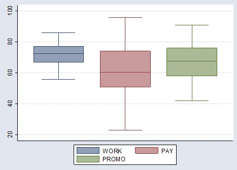
Figure 1: An Overall Box and Jenkins plot
We can then analyze the descriptive statistics table to translate the result above in a tabular form for the three aspects. The table will also help us to determine the specific values of mean, standard deviation, maximum, and minimum. Table 1 below shows that the mean for WORK satisfaction was highest with a value of 71.73529 followed by PROMO with 67.3825 and 62.48039 for PAY.
| Variable | Obs | Mean | Std.Dev. | Min | Max |
|---|---|---|---|---|---|
| WORK | 102 | 71.73529 | 7.303772 | 56 | 86 |
| PAY | 102 | 62.48039 | 16.39713 | 23 | 96 |
| PROMO | 102 | 67.38235 | 11.52874 | 42 | 91 |
Table 1: Overall Descriptive Statistics
Comparing Mean
We can use the bar graph to compare the overall mean satisfaction of the employees based on the three aspects. The bar graphs below confirm that WORK had the highest satisfaction average. Most employees were happy and satisfied with their WORK characteristics. There is therefore a need to improve the PAY and PROMO in order to get a higher value of overall satisfaction.
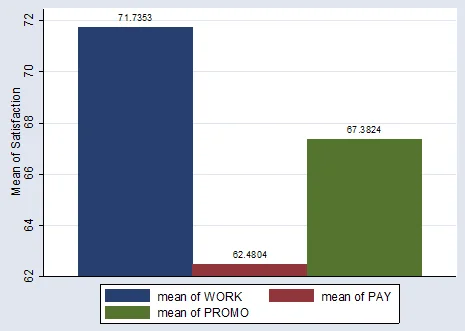
Figure 2: Overall Bar Graph to compare the Mean of the job characteristics
SECTION II: Measure of Variability of Employee Satisfaction
In order to help Nasee improve employee satisfaction, we analyze how spread the three aspects are. The spread can be analyzed using various methods including scatterplots, Box and Jenkins plots, and calculation of the interquartile range. From the Box and Jenkins in Figure 1 above, there was a higher spread in PAY satisfaction rating and the PROMO.
SECTION III: Analyzing Various Categories
Job Type
The summary statistic comparison of various Job types is shown in Table 2 – Table 5 below
| Variable | Obs | Mean | Std.Dev. | Min | Max |
|---|---|---|---|---|---|
| WORK | 22 | 69.09091 | 6.920701 | 60 | 82 |
| PAY | 22 | 57.77273 | 14.64153 | 29 | 86 |
| PROMO | 22 | 63.40909 | 10.83934 | 47 | 83 |
Table 2: Summary of Satisfaction effect for Clerical jobs
| Variable | Obs | Mean | Std.Dev. | Min | Max |
|---|---|---|---|---|---|
| WORK | 23 | 72.34783 | 7.333663 | 59 | 84 |
| PAY | 23 | 61.08696 | 12.47511 | 40 | 91 |
| PROMO | 23 | 68.65217 | 11.05609 | 48 | 83 |
Table 3: Summary of Satisfaction effect for Managerial jobs
| Variable | Obs | Mean | Std.Dev. | Min | Max |
|---|---|---|---|---|---|
| WORK | 17 | 77 | 7.331439 | 67 | 86 |
| PAY | 17 | 76 | 18.49324 | 40 | 96 |
| PROMO | 17 | 75.47059 | 11.12496 | 56 | 91 |
Table 4: Summary of Satisfaction effect for Supervisory jobs
| Variable | Obs | Mean | Std.Dev. | Min | Max |
|---|---|---|---|---|---|
| WORK | 40 | 70.6 | 6.511528 | 56 | 82 |
| PAY | 40 | 60.125 | 15.92693 | 23 | 92 |
| PROMO | 40 | 65.4 | 10.90001 | 42 | 91 |
Table 5: Summary of Satisfaction effect for technical jobs
Supervisory job type had the highest average satisfaction in all three aspects (WORK, PAY, and PROMO). We also realize that the mean for work was lowest for clerical job type. There was a very low satisfaction average for PAY, WORK, and PROMO satisfaction for the clerical job groups. The clerical group seems to be the unhappiest group and there is a need for the Nasee Inc. team to consider its improvement in PAY to improve its satisfaction. A clear graph showing the various differences for the average job groups is shown in Figure 3 below.
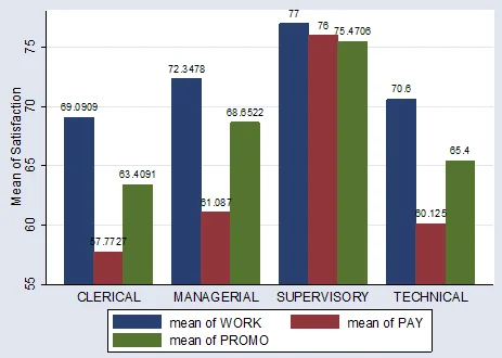
Figure 3: Bar Graphs showing the difference in means for various job groups
We can also display the spread using Box and Jenkins plots. From the Boxplot below, the highest range was seen in the PAY satisfaction for the technical group. The highest in this category is 92 and the lowest is 23. The highest spread is given by the PAY for the supervisory job group displayed by the highest standard deviation. We can also confirm that there was generally a lower spread in all four job groups for WORK satisfaction indicating agreement in the WORK satisfaction by all participants. The Box plot is shown in the figure below.
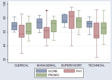
Figure 4: Box plot categorized by the job groups.
Educational Level
The educational Levels attained are categorized into three; High School Diploma (HSDIP), college level, and Bachelor's or master's Degree. The distribution of the sample size of the three categories is shown in Table 6 below.
| Education Level |
Count/Sample Size |
|---|---|
| High School Diploma (HSDIP) |
23 |
| College Level |
40 |
| Bachelors or Masters Degree |
39 |
Table 6: Counts of the various Education levels
The summary statistic tables below show the descriptive statistics of the three education levels attained.
| Variable | Obs | Mean | Std.Dev. | Min | Max |
|---|---|---|---|---|---|
| WORK | 39 | 77.58974 | 5.295072 | 60 | 86 |
| PAY | 39 | 78.35897 | 10.00128 | 60 | 96 |
| PROMO | 39 | 77.58974 | 7.070018 | 56 | 91 |
Table 7: Summary of Satisfaction Effect for Bachelors or Master’s Degree (BAMA)
| Variable | Obs | Mean | Std.Dev. | Min | Max |
|---|---|---|---|---|---|
| WORK | 40 | 68.525 | 5.643183 | 56 | 81 |
| PAY | 40 | 55.2 | 7.743318 | 40 | 76 |
| PROMO | 40 | 61.85 | 9.110574 | 47 | 81 |
Table 8: Summary of Satisfaction effect for college
| Variable | Obs | Mean | Std.Dev. | Min | Max |
|---|---|---|---|---|---|
| WORK | 23 | 67.3913 | 6.387055 | 56 | 79 |
| PAY | 23 | 48.21739 | 14.11626 | 23 | 90 |
| PROMO | 23 | 59.69565 | 8.63626 | 42 | 73 |
Table 9: Summary of Satisfaction Effect of High School Diploma (HSDIP)
From the tables, those who have attained a Bachelor's or master’s degree seem happy and highly satisfied with all three work characteristics. However, there was a wider spread in the PAY satisfaction rate compared to the other satisfaction aspects for the Bachelor's or Master’s attained. The employees who attained college as their highest education level, had almost equal satisfaction perception in all the aspects as shown by the lesser values of standard deviation. However, the PAY satisfaction average was lower compared to other satisfaction aspects.
Those who attained a high school diploma had a generally lower satisfaction rate in all aspects. In spite of the lower satisfaction rate in all aspects, there was a notably very lower rate in PAY satisfaction with an average of 48.2178 and a standard deviation of 14.11626 indicating a higher spread. A Box and Jenkins plot below shows the spread of the three groups and the three aspects.
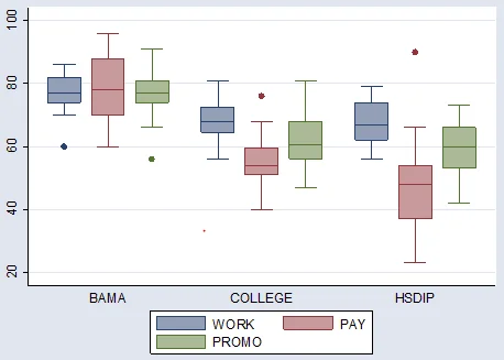
Figure 5: Box plot categorized by education level attained.
Location
The data was then categorized into the three locations; Location A, Location B, and Location C. The sample sizes of Location A, Location B, and Location C are 44, 32, and 26 respectively. The average rate of satisfaction was almost similar for the three groups with the lowest having 70.30769 and the highest at 73.54545. The spread was also lower as shown by a smaller sample variance. There was a lower satisfaction rate for employees in Locations B and C. There was notably a higher spread of pay satisfaction in all three location groups. The promotion satisfaction was average for all the groups with a high spread. The tables described above are shown.
| Variable | Obs | Mean | Std.Dev. | Min | Max |
|---|---|---|---|---|---|
| WORK | 44 | 73.54545 | 6.979887 | 60 | 86 |
| PAY | 44 | 67.90909 | 15.88449 | 38 | 94 |
| PROMO | 44 | 70.72727 | 11.6925 | 47 | 91 |
Table 10: Summary of Satisfaction for Employees in Location A
| Variable | Obs | Mean | Std.Dev. | Min | Max |
|---|---|---|---|---|---|
| WORK | 32 | 70.40625 | 7.024654 | 59 | 85 |
| PAY | 32 | 58.03125 | 16.37757 | 29 | 96 |
| PROMO | 32 | 64.71875 | 10.0426 | 48 | 88 |
Table 11: Summary of Satisfaction for Employees in Location B
| Variable | Obs | Mean | Std.Dev. | Min | Max |
|---|---|---|---|---|---|
| WORK | 26 | 70.30769 | 7.770556 | 56 | 85 |
| PAY | 26 | 58.76923 | 15.10313 | 23 | 92 |
| PROMO | 26 | 65 | 11.91973 | 42 | 81 |
Table 12: Summary of Satisfaction for Employees in Location C
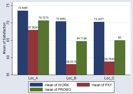
Figure 6: Bar graph for mean satisfaction categorized by Location
From the histogram above, there was a difference in mean PAY and mean of PROMO for Location A from Location B and Location C. However, there was a similarity in the mean of WORK for all three locations.
Conclusion
There can be general improvement in employee satisfaction if a few actions are taken. There is a need to provide an increase in PAY and opportunities for promotion for the employees with High school Diplomas, college degrees, Location B and Location C. Doing so will satisfy these employees more, making them feel valuable, showing them that even though they do not have a BAMA degree, they still get rewarded for their hard work and commitment in the company. There is no greater effect of employees’ satisfaction on WORK despite the location. However, Location has an impact on satisfaction for PAY and satisfaction for the opportunity of Promotion.