Problem Description:
This statistical analysis homework covers various statistical questions and tasks. We will provide solutions to these questions and briefly describe the approach taken for each.
Solution
Question 1
A study with a 70% power rate suggests that only 70 out of 100 statistical tests will actually find any true effects if there are any to be found in the 100 statistical tests. The projected Type II error threshold is 30% with a power of 70%. (1-0.7). The power of a study can be increased by increasing either the effect size, sample size or the significance level.
Question 2
a. Descriptive Statistics
library(haven)
data=read_sav('C:/Users/belak/Desktop/R/baguley_payne_2000.sav')
head(data)
summary(data)
| group | match | trials | percent_accuracy |
|---|---|---|---|
| Min. :0.0 | Min. : 1.00 | Min. : 8 | Min. : 12.50 |
| 1st Qu.:0.0 | 1st Qu.: 6.75 | 1st Qu.: 8 | 1st Qu.: 75.00 |
| Median :0.5 | Median :12.00 | Median :16 | Median : 87.50 |
| Mean :0.5 | Mean :13.43 | Mean :16 | Mean : 80.65 |
| 3rd Qu.:1.0 | 3rd Qu.:21.00 | 3rd Qu.:24 | 3rd Qu.: 91.67 |
| Max. :1.0 | Max. :24.00 | Max. :24 | Max. :100.00 |
b. The descriptive statistics is not appropriate for the “group” variable because it a categorical variable.
Question 4
a. Code and Plot
data=read_sav('C:/Users/belak/Desktop/R/Hayden_2005.sav')
head(data)
hist(data$days, xlab = "Days", main = "Histogram of Days")
hist(data$days, breaks=30, xlab = "Days"main="Histogram of Days With breaks=30")
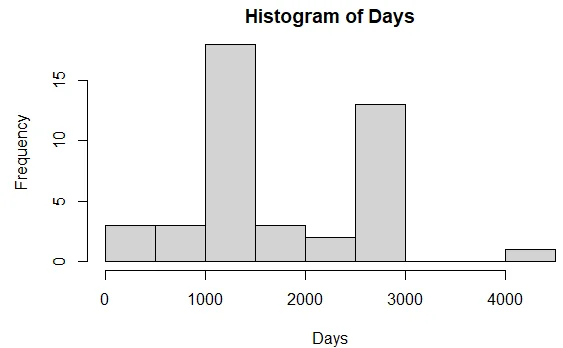
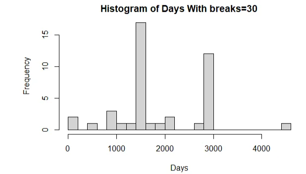
b. The histogram revealed that the days is normally distributed. It skewed to the left and hence the mean is less than the median.
Question 5
a. Code and Plot
data=read_sav('C:/Users/belak/Desktop/R/baguley_payne_2000.sav')
boxplot(data$percent_accuracy,ylab="Percent Accuracy",main="Boxplot of Percent Accuracy")
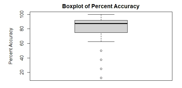
b. The box plot indicated that the percent accuracy is not normally distributed and negatively skewed. Hence the percent accuracy mean is less than the median.
c. Yes, there are outliers 4 outliers in the percent accuracy.
Question 6
a. Code and Plot
eclsk = read.csv("eclsk.csv")
head(eclsk)
lin.model <- lm (gen~math,eclsk)
plot(lin.model,2)
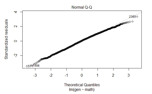
b. The Q-Q plot shows that the model residuals are normally distributed and hence, the normality of residual assumption was not violated.
Question 7
a. Code and Plot
eclsk = read.csv("eclsk.csv")
head(eclsk)
plot(eclsk$math,eclsk$gen, main='Regression for Math and Gen', xlab='Math',ylab='Gen')
abline(lm(gen~math,data=eclsk),col='red')
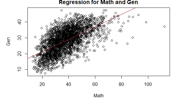
b. The scatter plot shows that there is linear relationship between the math and gen. Also, the assumption of homogeneity of variance is not violated.