Correlation and Regression
In the first question, we corrected inaccurate reasoning by a statistician who conducted a covariance test to determine the possible associations between two return series. Subsequent questions are all about regression, where we answer questions about predicting future Values, testing hypotheses, and others.
Correlation Analysis
Your colleague in a financial institution says that she has been tracking the movements of the monthly returns of Facebook and Amazon stock returns. Using data on these returns over the last 10 years, she says that she has computed the COVARIANCE between these two returns series and found that it is 0.00042. Since this COVARIANCE is so low and close to zero, she says that there does not seem to be any association between the two return series.
You tell her that (choose one of the following)
(i) her reasoning is faulty because….(give a brief reason)
(ii) her reasoning is correct because…(give a brief reason)
i. Her reasoning is faulty. Covariance can not be compared directly as it is unbounded and hence, the absolute value of covariance gives very little information. She should have calculated correlation which is covariance adjusted by the variance and then tested for significance to conclude anything.
correlation = cov(X,Y)/√(Var(X)×Var(Y) )
Regression
Is it possible that when you fit a simple regression model, the t-statistic for the slope coefficient is large (outside the range of (-2,2)), indicating that the X variable has a linear relationship with the Y variable, but that the R-squared value is quite low, say 8%?
(i) Yes (justify your choice with a short explanation)
(ii) No (justify your choice with a short explanation)
i. Yes. It may happen as the R-squared is the amount of variance explained. If the error or noise in the data is high, it can lead to low R-squared.
c) The regression of log(revenue of a firm) on log(R&D expenditure of firm) yields the following equation:
Log(Revenue) = 1.3 + 0.65 Log(R&D Expenditure)
In one sentence, interpret the value 0.65 of the slope in terms of the original variables “revenue of a firm” and “R&D expenditure of firm” (i.e. in terms of the unlogged variables)
Assuming natural log (i.e., base e log), the coefficient of 0.65 means that for each unit increase in R&D expenditure, the average increase in revenue is e^0.65=1.92 times.
2) The marketing manager of a large supermarket chain would like to determine the effect of shelf space and whether the product was placed at the front or back of the aisle on the sales of pet food. A random sample of 12 equal-sized stores was taken and the following variables were noted:
Y= sales=daily sales of the pet food (in thousands of $)
space=shelf space for the per food in square feet
location=0 if the pet food was placed at the back of the aisle
= 1 if the pet food was placed at the front of the aisle
The output from the fitted multiple regression is shown below
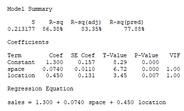
(i) The manager believes that for a fixed amount of shelf space, products placed at the front of the aisle sell more on average than products placed at the back. Is there evidence to support his belief? (Justify your answer with an appropriate number)
Yes. The data contains the evidence to support his claims as the t-test for significance of the location is statistically significant and the coefficient for the front is positive means if every other factor remains the same, the front location is expected to have higher sales than the back location.
(ii) Predict the daily sales of pet food if the product is placed at the front of the aisle and has 6 square feet of shelf space devoted to it.
Predictedsales = 1.300 + 0.0740 *6 + 0.450 *1=2.194K
The predicted sales are $2194.
(iii) For a store that places the pet food according to the plan in (iii) above (i.e. at the front of the aisle with 6 square feet of shelf space), what is the probability that the daily sales are less than $1550? (Justify your answer with an explanation)
Predictedsales = 1.300 + 0.0740 *6 + 0.450 *1=2.194
The predicted sales have Normal distribution with mean as 2.194 and SD as 0.2138.
The probability that sales are less than $1550 is:
P(Sales<1550)=P(z<(1.550-2.194)/0.2138)=0.00013
The probability is very low (p = 0.0001) that the daily sales are less than $1550.
(iv) An analyst in Ames, Iowa is provided exactly the same data for analysis and she fits the same multiple regression model as above. However, she codes her dummy variable for a location as follows:
location=1 if the product was placed at the back of the aisle
= 0 if the product was placed at the front of the aisle
She uses her model to predict daily sales of pet food if the product is placed at the front of the aisle and has 6 square feet of shelf space devoted to it. (i.e. the same characteristics as in part (ii) above)
(i) In what way would her predicted value differ from the value you obtained in (ii) above?
The predicted value will not be different. However, the coefficient s will vary. The intercept will now be equal to 1.3+0.450 and the coefficient of the X2 will be -0.450.
The predicted value remains the same.
(ii) What estimate would she get for the coefficient of location in her fitted regression equation?
The coefficients will be:
Intercept = 1.750
Coef X1 = 0.074
Coef X2 = -0.45
3) A real estate company has collected data on the following variables for several houses in a suburb of NYC:
Price: the price of the house (in $)
Story: the number of stories the house has
Baths: the number of baths the house has
A multiple regression fit to the above variables gave the following:
Regression Analysis: Price versus Story, Baths
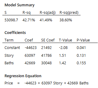
a) Which of the explanatory variables in the model are important on an individual basis, after accounting for the other variables?
The most important variable is Story. This is based on the p-values of the t-test. The p-value for Story is lower than Baths which makes it more effective. (Although, both of them are not statistically significant.)
b) Answer this question using the output on the earlier page as is, regardless of whatever you may have concluded in (a) above) The company has a house in the suburb that it wishes to sell. This house is 2 stories tall and has 1 bath. Based on the FULL MODEL on the previous page, make a suggestion for what price the agency should list the house at such that the agency is neither underselling the house nor overpricing it significantly. It is fine if your answer is a range of values.
Price = -44623 + 63097 Story + 42669 Baths
Price = -44623+63097×2+42669×1=124240.
The fitted value is $124,240 which is the suggested price.
If a range of values is required, a 95% Prediction interval is calculated as:
Lower Limit = 124,240 – 53098.7*1.96 = $ 20,166.55
Upper limit = 124,240 + 53098.7*1.96 = $ 228,313.5
The fitted value is suggested as sale price as this is the expected value of the price of the property. But if that is not the agreed price, a range of values given by the prediction interval captures the value of the property with 95% confidence.
c) When the analyst who carried out the analysis presents the model to the real estate agents at the company, the one agent says “I am quite puzzled by this. The variable “baths” has a t-statistic value within (-2,2), but I would definitely expect the number of bathrooms a house has to be related to its price
Give a brief but clear response to the agent that will clear up their confusion
Ans: The data indicates that a number of bathrooms may have an increasing relationship with the house price, but this variable is not able to explain a significant proportion of the variation in the house price which must be related through a lot of factors as well as it may have some interaction effect with another variable. This analysis is not proof of causation and hence, cannot be taken as such. More variables might be used to explain the trend in house prices and then this relationship can be captured better.