Regression and Predicting Test Scores Based on Other Attribute
This question corresponds to the dataset below with ten observations.
1. Make a scatter plot that shows how math aptitude predicts scores for both tests.
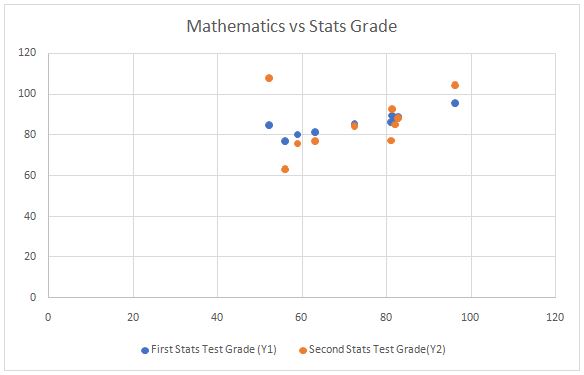
2. Describe the form of the relationships. Is there a linear pattern? Is the direction of the association positive or negative?
Ans: There is a positive relationship between Mathematics and both the tests. But, we can see a better linear pattern between Mathematics and the First test.
3. What is the equation of the OLS regression line for predicting both first and second test grades from math aptitude? Interpret the coefficients.
Ans: The OLS regression line between:
Mathematics and first test: (Y_1 ) ̂=65.549+0.321X
Mathematics and second test:(Y_1 ) ̂=65.552+0.321X
We can see both the above lines are almost the same. Here the intercept means the expected test score when the mathematics aptitude score is zero. The slope means the average increase in test scores when there is a 1 marks increase in mathematics aptitude score.
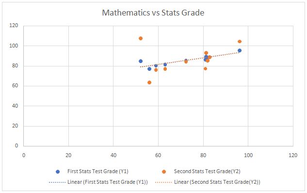
4. Draw a new scatterplot that includes labels for the points and the fitted line.
5. What is the Pearson correlation coefficient? Explain in simple language what this says about math aptitude and scores for each test. About what percent of the variation in test scores does math aptitude explain? Explain the difference between the “form/slope” of the relationship and the “fit” of the model to the data.
Ans: Pearson correlation coefficient is a test-statistics that measures the linear relationship between two continuous variables. The Correlation coefficient of math aptitude with test 1 and test 2 is 0.8768 and 0.3425 respectively. The percent of the variation in test scores that math aptitude explains is the square of correlation coefficients and multiplying with 100, i.e. 76.87% and 11.73% variation is explained for test 1 and test 2 respectively.
6. What is the predicted score on the first test for someone with a math aptitude of 80? What is the predicted score on the second test for someone with a math aptitude of 80?
Ans: As we can see the regression lines for the test are equal then the predicted score for both tests when someone has a score of 80 in math aptitude is 88.247.
7. With the information, you have available, conduct hypothesis tests for the significance of both the regression coefficients (t-test) and the overall fit of the regression models (F- test). Interpret your results. If you are using the computer, everything has already been calculated for you.
Ans: For test 1: The t-test statistic for the slope is 5.1568, and the F-statistic is 26.592. For both, the statistics are P-value is 0.0009. Thus, both the regression coefficient and the overall fit are statistically significant.
For test 2: The t-test statistic for the slope is 1.0312, and the F-statistic is 1.0633. For both, the statistics are P-value is 0.3326. Thus, both the regression coefficient and the overall fit are not statistically significant.
8. Using the residuals and/or the graph, which scores are the closest to being outliers? Do you think these results show that math aptitude is causally related to testing scores? Briefly assess the causal status of this relationship (feel free to speculate about possible alternative explanations).
Ans: Using the graph, a test score of 2 of 107.94 with a math score of 52.08 can be considered as an outlier. Due to the outlier, we can say that math aptitude is causally related to testing 2 scores.
Hypothetical Data for ten Observations on three variables
| Mathematics Aptitude (X) | First Stats Test Grades (Y1) | Second Stats Test Grades (Y2) |
| 52.08 | 85.01 | 107.94 |
| 55.96 | 77.10 | 63.4 |
| 58.92 | 80.39 | 76.05 |
| 63.07 | 81.68 | 77.17 |
| 72.39 | 85.56 | 84.59 |
| 81.05 | 86.36 | 77.46 |
| 81.34 | 89.56 | 93.09 |
| 82.03 | 88.22 | 85.50 |
| 82.79 | 89.07 | 88.78 |
| 96.31 | 95.73 | 104.71 |
2) For this question, use the Duncan Occupational Prestige data.
1. Estimate the bivariate regression predicting “prestige” as a function of “income.” Do the same for prestige as a function of education.
Ans: The regression equation for predicting “prestige” as a function of “income” is given by Prestige = 112.9821-0.5034*Income
The regression equation for predicting “prestige” as a function of “education” is given by Prestige = 7.5781 + 0.8818*education.
2. Carefully explain the meaning of each parameter estimate in both regression equations.
Ans: For first equation, the intercept value of 112.9821 means that average prestige when Income is 0, while the slope coefficient means that with 1 unit increase in income the prestige tends to decrease by 0.5034 on average.
For first equation, the intercept value of 7.5781 means that average prestige when Education is 0, while the slope coefficient means that with 1 unit increase in education the prestige tends to increase by 0.8818 on average.
3. Report the results for hypothesis tests of both the regression coefficient and the overall fit of the regression models. Interpret your results.
Ans: For the 1st equation: The t-test statistic for the slope is -0.4086, and the F-statistic is 0.1669. For both the statistics is P-value is 0.70.8. Thus, both regression coefficient and the overall fit are not statistically significant.
For the 2nd equation: The t-test statistic for the slope is 7.0864, and the F-statistic is 50.2173. For both the statistics is P-value is 0.0021. Thus, both regression coefficient and the overall fit are statistically significant.
4. Give the coefficient of determination (R2) for both equations. Based on these data, which variable (income or education) is a better predictor of occupational prestige?
Ans: The coefficient of determination for 1st and 2nd equation are 0.04 and 0.926 respectively. Thus, education is a better predictor of occupational prestige as it explains more proportion of variation in the occupational prestige.
Duncan Occupational Prestige Data
| Occupation | Income | Education | Prestige |
| Accountant | 62.00 | 86.00 | 82.00 |
| Author | 55.00 | 90.00 | 76.00 |
| Professor | 64.00 | 93.00 | 93.00 |
| Civil Engineer | 72.00 | 86.00 | 88.00 |
| Physician | 76.00 | 97.00 | 97.00 |
| RR Conductor | 76.00 | 34.00 | 38.00 |
| Store Manager | 42.00 | 44.00 | 45.00 |
| Mail Carrier | 48.00 | 55.00 | 34.00 |
| Carpenter | 21.00 | 23.00 | 33.00 |
| Machinist | 36.00 | 32.00 | 57.00 |
| Gs St. Attend | 15.00 | 29.00 | 10.00 |
| Taxi Driver | 9.00 | 19.00 | 10.00 |
| Barber | 16.00 | 26.00 | 20.00 |
| Cook | 14.00 | 22.00 | 16.00 |
| Janitor | 7.00 | 20.00 | 8.00 |