Brand Preferences on sweetness
1. Refer to the “Brand Preference” dataset(Brand.txt)
Column 1: Degree of brand liking(𝑌)
Column 2: Moisture content of the product
Column 3: Sweetness of the product
Code sweetness as a dummy variable.
(a). Regress degree of brand liking on sweetness only. Write down the estimated regression model.
Ans: Y = 68.625 + 4.375*Sweetness
(b). Compute the estimated mean degree of brand liking at each level of sweetness, i.e., what is the estimated mean degree of brand liking at sweetness level 2? At sweetness level 4?
Ans: At level 2, Y = 68.625 + 4.375*2 = 77.375
At level 4, Y = 68.625 + 4.375*4 = 86.125
(c). Interpret the intercept coefficient.
Ans: If the moisture content is zero, then the degree of brand liking is 68.625.
(d). Interpret the slope coefficient.
Ans: Increase in the degree of brand liking with one unit increase in the sweetness of the product.
(e). Is the slope coefficient significant? State the null, alternative, decision rule, and conclusion.
Ans: H_0:β=0 vs H_a:β≠0. We reject the null hypothesis if the p-value is less than 0.05. Here the p-value is 0.13, thus we fail to reject the null hypothesis. Hence we conclude that there’s not enough evidence to support the claim that the slope coefficient is significant.
2. Refer to the “Brand Preference” dataset. Code sweetness (𝑿𝟐) as a dummy variable.
(a). Fit a multiple regression model with moisture content, sweetness, and their interaction.
(b). Write down the estimated regression equation at each sweetness level.
Ans: The regression equation is: Y = 27.15 + 5.925*X1 + 7.875*X2 – 0.5*X1*X2
(c). Interpret the slope coefficient in each estimated regression equation in Part (b).
Ans: Coefficient of X1 = Keeping X2=0, with each unit increase in X1, Y increases by 27.15.
Coefficient of X2 = Keeping X1=0, with each unit increase in X2, Y increases by 7.875.
(d). Is the interaction coefficient significant at 𝛼 = 5%? State the null, alternative, decision rule, conclusion.
Ans: H_0:β_12=0 vs H_a:β_12≠0. We reject the null hypothesis if the p-value is less than 0.05. Here the p-value is 0.097, thus we fail to reject the null hypothesis. Hence, we conclude that there’s not enough evidence to support the claim that the interaction coefficient is significant.
(e). If your answer is NO in Part (d), drop the interaction term and rerun the model. Write down the new estimated regression equation at each sweetness level.
Ans: The new model is: Y = 37.65 + 4.425*X1 + 4.375*X2.
3. Refer to the “Assessed Valuations” dataset (Value.txt)
Column 1: Selling price (𝑌), in thousands of dollars.
Column 2: Assessed valuation (𝑋1), in thousands of dollars (continuous)
Column3: Lot location (𝑋2), coded as 1 for corner lots and 0 for non-corner lots (already dummy)
(a). Regress selling price on lot location only. Write down the estimated regression equation.
Ans :Y = 68.625 + 4.375*X2
(b). Based on your regression result in Part (a) what is the estimated mean selling price for corner lots? For non-corner lots?
Ans: For corner lots: Y = 68.625 + 4.375* 1 = 73
For non-corner lots: 68.625 + 4.375*0 = 68.625
(c). Based on your regression result in Part (a), what is the estimated difference in selling price between corner and non-corner lots? Is this difference statistically significant?
Ans: The difference is the slope coefficient, which is 4.375. No. the difference is not statistically significant as the p-value for the test is 0.13.
(d). Regress selling price on assessed valuation, lot location, and the interaction. Write down the estimated regression equation for corner lots, and for non-corner lots respectively.
Ans: Y = 27.15 + 5.925*X1 + 7.875*X2 – 0.5*X1*X2 is the general equation
For corner lots: Y = 27.15 + 5.25* X1 + 7.875 – 0.5*X1 => Y = 35.025 + 4.75*X1
For non-corner lots: Y = 27.15 + 5.25*X1
(e). Plot the estimated regression lines for the two groups and describe their differences.
Ans: The two lines are:
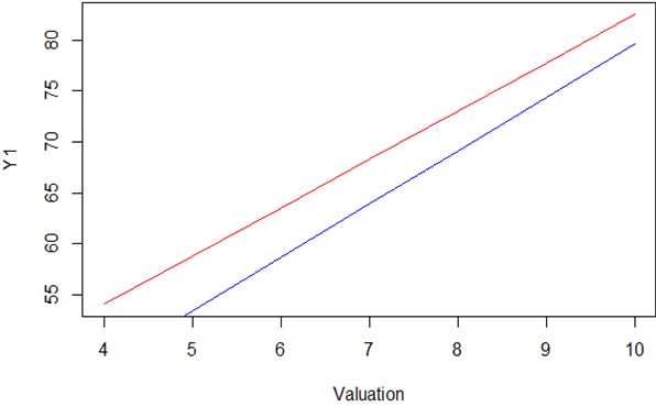
Where red represents the corner lots line and blue represents the non-corner lots.
Here not much difference in the lines is observed, though we can say that the red line is above the blue line in the given range of X1.
(f). Based on your regression in Part (d), test whether the regression lines for corner lots and non-corner lots are parallel. State the null, alternative, decision rule, and conclusion.
Ans:H_0:β_12=0 vs H_a:β_12≠0. We reject the null hypothesis if the p-value is less than 0.05. Here the p-value is 0.097, thus we fail to reject the null hypothesis. Hence, we conclude that there’s not enough evidence to support the claim that the interaction coefficient is significant