Various SAS Topics
Topics: Correlation, Simple and Multiple Linear Regression, Simple and Multiple Logistic Regression, ANOVA, ANCOVA
Q.1.
The following SAS output shows the results of an analysis where the response variable mean hemoglobin level in g/dl (H level) is continuous. It is of interest to see how the H level changes with gender (1- male, 0-female). It is also known from the past research that H level is also affected by age in yrs. So it should be controlled in the model.
(a) What statistical model was used to get this output?
(b) Interpret the results based on the above output.
(c) Based on the first table, Age is not a significant predictor in this model, do you keep or remove it from the analysis? why?
Q1 Ans
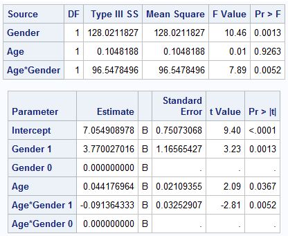
a. The statistical model that was used for this is ANCOVA (Analysis of Covariance). There is one continuous covariate and one categorical variable that aims to test the difference of H level in gender.
b. The result of the model is statistically significant for both gender and the interaction of age and gender. It is evident from the output that the H level has a significantly different level for males and females and that this difference changes with age.
The gender is statistically significant with a p-value =0.0013 but the main effect of age is not significant with a p-value being 0.9263. The interaction term, however, is statistically significant with a p-value being 0.0052.
c. No. Clearly, the interaction term of age and gender is not insignificant and hence, age should not be removed from the main model as the effect of gender varies with each level of age. Predictions based on values of age and gender will need both the direct and the interaction coefficients to be reliable.
Q.2.
The following output shows the OR estimates of cardiovascular disease (CVD) status- Yes and No.
(a) What statistical model was used to get this output?
(b) Which of the above predictors are significant in determining the CVD status?
(c) Race is a variable where 1- Others, 2-AA, and 3-Whites. Interpret the result of Race
(d) Interpret the result on weight.
Q2 Ans:
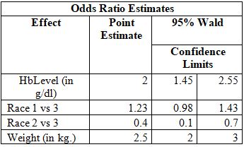
a. The model used for this analysis was logistic regression.
b. All the variables are significant predictors in determining CVD, namely HbLevels, Race, and weight since for each effect, the confidence intervals do not contain 0.
c. The Race variable has 3 levels in which 2-White is the reference. The interpretation would be: Given HbLevel and Weight, an individual’s odds of having CVD increases by 1.23 amount on an average if the person is from a race Other than White and AA as compared to the odds if person wereWhite. However, if a person is an AA, the odds of having CVD increases by 0.4 on an average, as compared to the odds if the same person was White.
d. Weight is a statistically significant variable with a coefficient of 2.5. This means on average, for each 1kg increase in weight, the odds of having CVD increases by 2.5.
Q.3.
The following SAS output shows the results for fitting a statistical model to predict the length of hospital stay (in hours.). The variables included in the table are infection status-1- Yes, 0-No; and CVD status-1-Yes, 0-No.
(a) What statistical model was used to fit hospital stay?
(b) How do you interpret the parameter estimate of the intercept?
(c) Interpret the results based on the second table.
(d) How can you improve this model?
Q3 Ans:
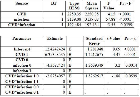
a. The model that was used here is two-way ANOVA with interaction. This is because the aim was to test if length of hospital stay (a quantitative variable) depends on CVD status and infection status which are both categorical variables.
b. Intercept is 12.42 which means that if both CVD status and infection is 0, average length of hospital stay is 12.42.
c. The second table gives us result for the main effects of CVD, and infection as well as the interaction terms. The interpretations are following:
i. CVD: The CVD status effect is significant with p-value being <0.001. The coefficient 6.35 for CVD level 1 show that if an individual has CVD, the length of hospital stay is, on an average, 6.35 hours more than the individual with no CVD given an infection status.
ii. Infection: The Infectionstatus effect is significant with p-value being 0.0014. The coefficient -4.368 for Infectionlevel 1 show that if an individual has Infection, the length of hospital stay is, on an average, 4.368 hours less than the individual with no Infectiongiven an CVD status.
iii. The interaction term between CVD and Infection is not significant with p-value 0.0599 at 5% level of significance. The coefficient of -2.875 indicates that if an individual has both CVD and infection then on an average, length of hospital stay reduce by 2.875 hours.
d. The model can be improved by adding few more relevant variables like age, hospital charges, financial status, and other health factors, and other factors which can realistically affect the hospital stay. We should also include the interaction term for two- and three-way interactions after adding more relevant variables.
Q.4
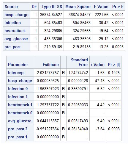
The following SAS output is obtained by fitting the best model to predict length of hospital stay (hours). Other variables in the table are- hosp_charge- hospital cost(in $); infection-1-Yes, 0- No; heartattack-1- Yes, 0-No; avg_glucose- average blood glucose level, pre_post- 1 pre intervention period, 2- post intervention period.
(a) Is this a good model, justify with reasons?
(b) Interpret the parameter estimate of hosp_charge in terms of $10,000.
(c) Write down the model in linear regression form with dummy variables.
(d) Write down the fitted model in linear regression form with dummy variables.
(e) What is the expected length of stay for a person who paid $15000, had infection but no heartattack, average glucose level of 140 and was from post period.
(f) Carry out a five step hypothesis testing on avg_glucose.
(g) Based on above tables, write a brief report of no more than 200 words.
Q4 Ans:
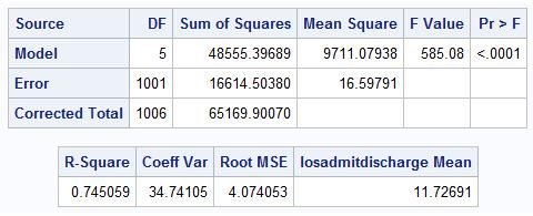
The model fitted is good as the R2 of the model is 0.745 which is high with all of the variables being statistically significant.
The coefficient of hospital charge is $0.000059 means that for each $10,000 increase in hospital charges, the length of hospital stay increases by 0.59 hours on an average.
The regression model fitted is given below:
Hospital Stay=α+β_1×Hospital Charge+β_2×I(Infection=1)+β_3×I(Heart Attack=1)+β_4×Avregae Glucose+β_5×I(Post Intervention=TRUE),
where I is an indicator function which takes value 1 when condition is true and 0 if false.
The regression model fitted is given below:
Hospital Stay= -2.031273757+0.000059×Hospital Charge-1.968397023×I(Infection=1)+1.293757722×I(Heart Attack=1)+0.044115357×Avregae Glucose-0.851227664×I(Post Intervention=TRUE),
where I is an indicator function which takes value 1 when condition is true and 0 if false.
The expected length of stay is:
Hospital Stay= -2.031273757+0.000059×15000-1.968397023×1+1.293757722×0+0.044115357×140-0.851227664×1
Hence, Hospital Stay=2.210251536 hours
The 5-step hypothesis testing is done below:
Test: We shall use t-test for the significant of coefficient.
Hypothesis:
H_0: β_4=0 vs H_1: β_4≠0
The level of significance is kept at 5%. The cutoff value is decided by t(1001) which can be approximated closely by normal distribution and hence, we would simply use normal distribution. The cutoff value is 1.96
Test Statistic calculation
t=0.044115357/0.00817493=5.4
P-value = 0.0000000666
Decision: reject the null hypothesis in favor of alternative.
Conclusion: We have sufficient evidence to claim that the effect of average glucose on hospital stay is not 0.
The analysis was done to predict the length of hospital stay by using few variables like hospital charges, infection status, heart attack indicator, average blood glucose and if the period was pre- or post-intervention. It was found that all of these variables turned out to be statistically significant with Heart attack, average blood glucose, and Hospital charges having increasing effect while infection, and intervention having decreasing effect. The model overall is statistically significant in predicting the length of hospital using these explanatory variables with good R2 of 0.745 which means that 74.5% of variance in length of hospital stay was explained by the predictor variables. The most significant variable among these was hospital charge where the estimated effect was found be for each $10,000 increase in hospital charges, the length of hospital stay increases by 0.59 hours on an average. The intercept however, was not found to be significant.