Assignment on finding the probability of selecting a certain phenomenon, Mean, Standard deviation.
MA 150 Final Exam Review
Q1)
(a)
P (Selecting a residential student that is a sophomore) = 410/1510 = 41/151 = 0.2715
(b)
P (Selecting a residential student who has a car on campus) = 486/1510 = 0.3218
(c)
P (Selecting residential student is either sophomore or has a car) = (410 + 186 + 220)/1510
P (Selecting residential student is either sophomore or has a car) = 0.5404
(d)
P (Student has car| Student is a senior) = 220/255 = 0.8627
(e)
P (Student is a freshman), P (Student who has a car on campus) are mutually exclusive events, as the probability of both events occurring at the same time is equal to zero.
Q2)
Population mean = 30.5 months
Population standard deviation = 1.25 months
(a)
Z (33) = (33 – 30.5)/1.25 = 2
Therefore, time to failure of 33 months is 2 standard deviation greater than the population average.
(b)
P (30 < Time to failure < 31) = P ((30 – 30.5)/1.25 < Z < (31 – 30.5)/1.25) = P (-0.4 < Z < 0.4)
P (-0.4 < Z < 0.4) = P (Z < 0.4) - P (Z < -0.4) = 0.3108
(c)
P (Time to failure < 24) = P ((24 – 30.5)/1.25 < Z) = P (Z > -5.20) = 9.964*10-8
(d)
Z value of 95th percentile = 1.644854
Time to failure of 95th percentile = 30.5 + 1.644854*1.25 = 32.55607 months
Q3)
(a)
Sample average = Sum of wait times/6 = 37.5/6 = 6.25 minutes
Sample standard deviation = SQRT((X-Mean)2/5) = 1.4167
(b)
95% confidence interval = (Mean – tc*SD/SQRT(N), Mean + tc*SD/SQRT(N))
Value of tc at 95% confidence, df = 5 is 2.5706
95% confidence interval = (6.25 – 2.5706*1.4167/sqrt(6), 6.25 + 2.5706*1.4167/sqrt(6))
95% confidence interval = (4.763254 minutes, 7.736746 minutes)
(c)
I think the bank’s advertising is not honest, as the bank’s claim of average wait times being less than 4 minutes isn’t a part of the 95% confidence interval computed in (b).
Q4)
Population average = $35,000
Population standard deviation = $3,200
Sample average = Sum of all salaries/10 = $37,500
Null hypothesis: Average starting salaries of new graduates from State University is equal to $35,000
Alternate hypothesis: Average starting salaries of new graduates from State University is not equal to $35,000
We will use the one sample Z test to test the hypothesis as the population standard deviation is known.
Z = (Mean – 35000)/(SD/SQRT(N)) = (37500 -35000)/(3200/sqrt(10)) = 2.4705
P-value = 0.0135 > 0.01
Therefore, at 0.01 significance level, we fail to reject the null hypothesis that the average starting salaries of new graduates from State University is equal to $35,000.
We conclude that there is insufficient evidence to support the University placement office’s suspicion that the average starting salary has changed from $35,000
Q5)
(a)
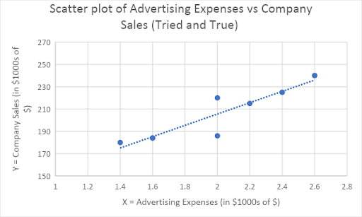
The scatterplot above, shows the data points with the regression line.
(b)
Predicted company sales for company with x = 2.0
Predicted company sales = 104.1 + 50.7*2 = 104.1+ 101.4 = $205,500
(c)
Residual for the (2,220) coordinate = $220,000 - $205,500 = $14,500
The model has under predicted the company’s sales
(d)
The value of the slope is 50.7, which means for each $1000 increase in the company’s advertising expenses, the value of the company’s sales increases by $50,700
(e)
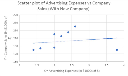
The scatterplot with the regression line with the addition of new company is shown above.
(f)
The New Company is an influential observation as it has significantly altered the slope and R2 value of the regression line
(g)
The “With New Company” line is not a good predictor of Company Sales, as the value of R2 is pretty low, compared to the earlier line.
Q6)
(a)
Mean of X-bar = 8
Standard deviation of X-bar = 2.25/SQRT(15) = 0.5809
(b)
The probability distribution of the sample mean, x-bar is likely to be normally distributed, as the underlying data is normally distributed.
(c)
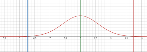
The lines indicate the location of mean and three standard deviations above and below the mean.
(d)
P (Sample mean > 10) = P(Z > (10 – 8 )/(0.5809)) = P (Z > 3.4426) = 0.000288
(e)
P (Sample mean > 10) = P(Z > (10 – 8 )/(2.25/sqrt(50)) = P (Z > 2/0.3181981) = P (Z > 6.28)
P (Z > 6.28) = 1.635*10-10
(f)
The event in part (d) is more likely compared to event in part (e).
Q7)
Null hypothesis: Mean time spent watching television by women is greater than or equal to mean time spent watching television by men
Alternate hypothesis: Mean time spent watching television by women is less than the mean time spent watching television by men
To test the hypothesis, the independent samples t-test will be used. We will use a one tailed t-test, with the critical region on the left side of the distribution to test the hypothesis.
The critical value of t-statistic, at 0.05 significance level, df = 14 + 17 – 2 = 29 is -1.699127
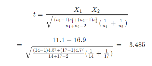
As the computed value of t-statistic is less than the critical value of t-statistic, we reject the null hypothesis and conclude that there is sufficient evidence to support the hypothesis that the mean time spent watching television by women is less than the mean time spent watching television by men
Q8)
(a)
The five number summary for Barry Bonds is (16, 25, 35.50, 45.25, 73). The five number summary for Sammy Sosa is (4, 15, 36, 50, 66).
(b)
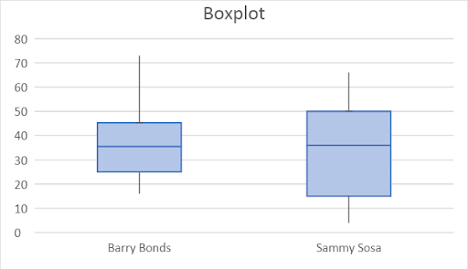
Boxplots are shown above.
(c)
The range for Barry Bonds = 57
The range for Sammy Sosa = 62
IQR for Barry Bonds = 20.25
IQR for Sammy Sosa = 35
(d)
The center for Barry Bonds is 35.50, compared to 36 for Sammy Sosa. The shape of Sammy Sosa's distribution is similar to that of Barry Bonds. The spread of Sammy Sosa is greater than that of Barry Bonds, as the value of IQR is greater for Sammy Sosa compared to Barry Bonds.
(e)
Upper fence for Barry Bonds = Q3 + 1.5*IQR = 45.25 + 1.5*20.25 = 75.625