Problem Description: Bonus Problem A
In this STATA assignment, we tackle two distinct statistical problems. The first problem, referred to as Bonus Problem A, focuses on estimating the prevalence of exit site infection among patients who received percutaneous placed catheter treatment. We also determine a 95% confidence interval for this prevalence. The second part of this problem involves Bonus Problem B, which delves into the evaluation of mortality rates between early and late start groups, using hypothesis testing.
Solution
Bonus Problem A
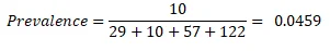
A.1 Point estimate of prevalence
A. 2 95% CI for the prevalence
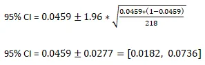
A. 3 The Point estimate of prevalence of exit site infection among patients who received the percutaneous placed catheter treatment is 0.0459 (4.59%). We are 95% confident that the prevalence in the population of exit site infection among patients who received the percutaneous placed catheter treatment lies between 0.0182 (1.82%) and 0.0736 (7.36%).
Bonus Problem B
B.1 The variable of interest is mortality rate
B.2 Null hypothesis: there is no difference between the mortality rate of both early and late start groups.
Alternative hypothesis: there is a difference between the mortality rate of both early and late start groups.
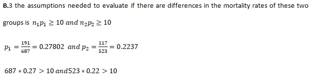
B.4 We use 2-sample Z-test for proportions to evaluate if there are differences in the mortality rates of these two groups
B.5 Decision rule for the test statistic.
Reject the null hypothesis if the Z calculated is greater than the critical value, otherwise, do not reject.
B.6 Calculate the test statistic by hand, report the degrees of freedom (if applicable) using the critical value method to test the hypothesis of interest and conclude.
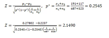
Critical value = 1.96
Since the Z calculated (2.149)is greater than the critical value (1.96), we reject the null hypothesis and conclude that there is a significant difference between the mortality rates of both early and late start groups
B.7 Calculate the test statistic in Stata or any other statistical software, report the degrees of freedom (if applicable) using the critical value method to test the hypothesis of interest and conclude
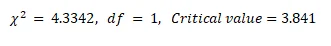
Since the test statistic calculated (2.149) ) is greater than the critical value (3.841), we reject the null hypothesis and conclude that there is a significant difference between the mortality rates of both early and late start groups.
B.8 Using the estimated test statistic, please estimate and report the p-value associated with the test statistic.
p-value = 0.0316
B.9 Conclude and interpret your results
Since the p-value (0.0316) is less than the significance level (0.05), we reject the null hypothesis and conclude that there is a significant difference between the mortality rates of both early and late start groups.
Problem 1
Observed
| Use of OC oracon | |||
|---|---|---|---|
| Yes | No | Total | |
| endometrial-cancer | 6 | 104 | 110 |
| Control | 6 | 184 | 190 |
| Total | 12 | 288 | 300 |
Expected
| Use of OC oracon | |||
|---|---|---|---|
| Yes | No | Total | |
| endometrial-cancer | 4.4 | 105.6 | 110 |
| Control | 7.6 | 182.4 | 190 |
| Total | 12 | 288 | 300 |
Null hypothesis: there is no association between the use of OC Oracon and the prevalence of endometrial cancer.
Alternative hypothesis: there is an association between the use of OC Oracon and the prevalence of endometrial cancer.
tabi 6 104\6 184, chi2 exact
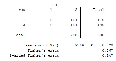
Since the p-value (0.328) is greater than the significance level (0.05), we do not reject the null hypothesis and conclude that there is no association between the use of OC Oracon and the prevalence of endometrial cancer.
Problem 2
We use exact method for McNemar test when we have a paired binomial or nominal data when the sample size of discordant is small. It is use when one is interested in finding a change in proportion for the paired data.
We use chi-square test of independence when we have two nominal variables, each with two or more possible values.
Problem 3
Construct the observed and expected 2X2 tables.
Observed
| Group | |||
|---|---|---|---|
| children with the disease at baseline | children with otorrhea after 2 weeks | Total | |
| Antibiotic ear drops | 76 | 4 | 80 |
| Oral antibiotics | 77 | 34 | 111 |
| Total | 153 | 38 | 191 |
Expected
| Group | |||
|---|---|---|---|
| children with the disease at baseline | children with otorrhea after 2 weeks | Total | |
| Antibiotic ear drops | 64.08377 | 15.91623 | 80 |
| Oral antibiotics | 88.91623 | 22.08377 | 111 |
| Total | 153 | 38 | 191 |
The variable of interest is the prevalence of otorrhea
The parameter of interest is proportions of children who still reported having otorrhea for the two treatment groups.
Null and Alternative hypotheses
- Null hypothesis: there is no difference between the proportions of children who still reported having otorrhea for the two treatment groups.
- Alternative hypothesis: there is a difference between the proportions of children who still reported having otorrhea for the two treatment groups.
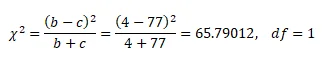
We are to use McNermar’s test for marginal homogeneity, we have sufficiently large number of discordant,
Decision rule: reject the null hypothesis if the test statistic is greater than the critical value.
p-value= 0.000
We reject the null hypothesis and conclude that there is a difference between the proportions of children who still reported having otorrhea for the two treatment groups.
Problem 4
- Null hypothesis: The proportion of hens whose biliary secretions increased is equal across the different hormones.
- Alternative hypothesis: The proportion of hens whose biliary secretions increased is different across the different hormones.
I sorted the ID and there are multiple replicated hormone records for each ID, the 2nd observation for the records with same id and hormone is retained. 62 observations were retained out of the 97 observations. The Stata commands for the categories is tabulate changebilisec hormone.
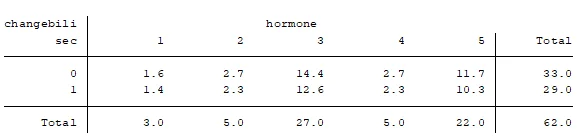
The correct test statistic to test the hypothesis of interest is Fisher's exact test of independence since expected frequencies in some of the cells are less than 5.
Fisher's exact = 0.189
Since the p-value (0.189) is greater than the significance level (0.05), we do not reject the null hypothesis and conclude that the proportion of hens whose biliary secretions increased is equal across the different hormones.
Problem 5
- Null hypothesis: The proportions of no tonsillectomy are the same for patients and siblings
- Alternative hypothesis: The proportions of no tonsillectomy are different for patients and siblings.
The variable of interest is the number of patients and siblings with no tonsillectomy.
The parameter of interest is the proportion of patients and siblings with no tonsillectomy.
Identify and state the test statistic.
The test statistic is McNermar’s test statistic.
Decision rule: reject the null hypothesis if the test statistic is greater than the critical value
5.6. [3 points] Calculate the test statistic in stata or statistical software and report the degrees of freedom (if applicable) to test the hypothesis of interest.
McNemar's chi2(1) = 1.32 Prob > chi2 = 0.2513
Since the p-value (0.2513) is greater than the significance level (0.05), we do not reject the null hypothesis and conclude that the proportions of no tonsillectomy are the same for patients and siblings.
Problem 6
- Null hypothesis: There is no association between a genetic risk score and macular degeneration
- Alternative: There is an association between a genetic risk score and macular degeneration
The variable of interest is number of women with macular degeneration, the parameter of interest is odds ratio
Chi square test is used
Decision rule: reject the null hypothesis if the test statistic is greater than the critical value.
6.6. [2 points] Calculate the test statistic and report the degrees of freedom (if applicable) using the critical value method to test the hypothesis of interest.
chi2 = 3.87, df = 1
Critical value = 3.841
Prob > chi2 = 0.0491
Since the chi2 (3.87) calculated is greater than the critical value (3.841), we reject the null hypothesis and conclude that there is an association between a genetic risk score and macular degeneration. Hence, there is a trend in the risk