Problem Description:
The aim of linear regression homework is to establish a relationship between temperature and various meteorological variables in order to predict the temperature for the year 2022 using linear regression. We focus on London's climate, characterized by mild winters and temperate summers with average daytime temperatures ranging from 5.5°C in January to 18°C in July. We have 60 days' worth of weather data from 2021 and will utilize linear regression to estimate the temperature for 2022.
Solution
df1=read.csv("2021 Weather.csv",header=T)
dim(df1)
## [1] 60 6
| Temperature | Humidity | Wind | Pressure |
|---|---|---|---|
| Min. :12.00 | Min. :52.00 | Min. : 4.400 | Min. :29.80 |
| 1st Qu.:14.00 | 1st Qu.:66.10 | 1st Qu.: 6.350 | 1st Qu.:29.98 |
| Median :15.80 | Median :71.70 | Median : 7.750 | Median :30.05 |
| Mean :16.30 | Mean :72.78 | Mean : 8.210 | Mean :30.04 |
| 3rd Qu.:18.05 | 3rd Qu.:80.97 | 3rd Qu.: 9.425 | 3rd Qu.:30.10 |
| Max. :22.70 | Max. :93.90 | Max. :16.000 | Max. :30.30 |
Location
Length: 60
Class: character
Mode: character
hist(df1$Temperature)
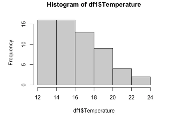
hist(log(df1$Temperature))
As we can see the histogram of the temperature is not bell shaped i.e. does not follow the normal distribution we decided to use the log transformation which fitted the normal assumption well.We also performed a Shapiro test which has ascertained the normality of the data at 0.01 significance level.

df1$logt=log(df1$Temperature)
##
## Shapiro-Wilk normality test
##
## data: df1$logt
## W = 0.95953, p-value = 0.04462
lm1=lm(logt~Day+Humidity+Wind+Pressure+Location,data=df1)
summary(lm1)
##
## Call:
## lm(formula = logt ~ Day + Humidity + Wind + Pressure + Location,
## data = df1)
##
## Residuals:
## Min 1Q Median 3Q Max
## -0.246550 -0.082393 -0.008758 0.094237 0.216646
##
## Coefficients:
## Estimate Std. Error t value Pr(>|t|)
## (Intercept) 6.9119735 4.3751610 1.580 0.11999
## Day -0.0020374 0.0020181 -1.010 0.31720
## Humidity -0.0052711 0.0018391 -2.866 0.00591 **
## Wind -0.0002759 0.0068214 -0.040 0.96788
## Pressure -0.1266854 0.1432891 -0.884 0.38055
## LocationLondon 0.1800490 0.0324158 5.554 8.74e-07 ***
## ---
## Signif. codes: 0 '***' 0.001 '**' 0.01 '*' 0.05 '.' 0.1 ' ' 1
##
## Residual standard error: 0.1172 on 54 degrees of freedom
## Multiple R-squared: 0.5191, Adjusted R-squared: 0.4746
## F-statistic: 11.66 on 5 and 54 DF, p-value: 1.152e-07
par(mfrow=c(2,2))
plot(lm1)
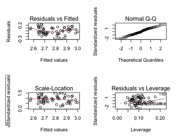
Next we fitted a regression model with log of the temperature of the outcome and all the variables as independent variables as the number of variables are less we haven’t used any variable selection technique. Day of the month and location has been shown as statistically significant variable in the linear regression model. In order to check the functioning of the regression we have plotted the diagnostics of the plot. The regression diagnostics plot fares well with the regression assumption of normality, independence and equal variance.
dft=read.csv("2022 Weather.csv")
temp=dft[,2]
dft=dft[,-2]
pred=predict(lm1,newdata=dft)
ptemp=exp(pred)
mse=mean((temp-ptemp)^2)
mse
## [1] 3.9688
At last, we have predicted the temperature of 2022 using same regression model and used MSE as the measure of performance, as we can see that the MSE is very low, we are pretty much satisfied with the performance of the model.