Problem Statement:
A STATA analysis homework that explores the relationships between various variables in the context of opioid-related deaths and healthcare expenditure in the United States. These variables are drawn from different sources, and they span the years 2000-2020. Here is a brief overview of the key variables and their sources:
Solution
Data Description
The name and the description of each variable has been shown below in Table 1 with their data sources.
Table 1
Variables and Data Sources
| Name | Variable | Description | Source | |
|---|---|---|---|---|
| medicareinmillion | Medicare Spending | Total Medicare spending by state | CMS GOV | |
| medicaid | Medicaid Spending | Total Medicaid spending by state | Medicaid GOV Years: 2000-2020 |
|
| tcmcaremcaidml | Medicare/Medicaid | Medicare/Medicaid costs in millions | ||
| tcmcaremcaidmladj | Medicare/Medicaid adjusted | Medicare/Medicaid costs in millions, adjusted | ||
| oddeaths | Overdoses | Opioid Overdose Deaths | Kaiser Family Foundation | |
| population | Population | State Population Estimates | US Census Bureau | |
| medinc | Median Household Income | Median Family Income | US Census Bureau | |
| mdehhincadj | Adjusted Median Household Income | Median household in income in millions adjusted for 2020 | ||
| stategdp | State GDP | Annual Gross Domestic Product by state | US Bureau of Economic Analysis | |
| unemprate | Unemployment Rate | Average annual unemployment rates by state | US Bureau of Labor Statistics | |
| lfpr | Labor Force Participation Rate | Percent of civilian noninstitutional population 16+ of age working or actively seeking work | US Bureau of Labor Statistics | |
| prctinsured | Percent Insured | Percent of population with Health Insurance Coverage | US Census Bureau for years 1999-2012 and 2008-2020 | |
| pchsgrad | Percent high school graduates | Percent of population with a high school degree or higher | US Census Bureau Educational Attainment | |
| pcgdpmanu | Manufacturing in GDP, % | % GDP in the manufacturing sector in each state | Data file given by professor | |
| pcempmanu | Manufacturing Employment, % | % of employment in the manufacturing sector in each state | Data file given by professor | |
| Phase2 | Dummy Variable | Dummy variable = 1, if year is later than 2009; = 0, if year is 2009 or earlier | Created in STATA | |
| prescript | Prescription Rate | Opioid prescriptions dispensed per 100 persons per year | Centers for Disease Control and Prevention | |
| cpi | Consumer Price Index | Consumer Price Index, measure of inflation rate | … |
After describing the variable names and its sources, now we can get to know our data. Table 2 gives a summary statistic of the numerical variables in the dataset.
Table 2
Summary Statistics of Numerical Variables
| Variable | Obs | Mean | Std. Dev. | Min | Max |
|---|---|---|---|---|---|
| stateid | 0 | ||||
| year | 1.071 | 2010 | 6.05813 | 2000 | 2020 |
| medicarein-n | 1.071 | 9405,177 | 11727,76 | 216 | 86833 |
| medicade | 1.071 | 7.93e+09 | 1.15e+10 | 1,05e+08 | 9,78e+10 |
| oddeaths | 1.071 | 519,6671 | 675,8681 | 10 | 5508 |
| population | 1.071 | 6037820 | 6782164 | 494300 | 3,94e+07 |
| medinc | 1.071 | 52509.63 | 11683,31 | 29359 | 95572 |
| stategdp | 1.071 | 303082.5 | 388213,1 | 17152,5 | 3042694 |
| 1fpr | 1.071 | 65,4732 | 4.263374 | 53,3 | 75,3 |
| unemprate | 1.071 | 5,600187 | 2,039548 | 2,1 | 13,8 |
| prctinsured | 1.071 | 88.18487 | 4,382695 | 74.5 | 97,5 |
| pchsgrad | 1.071 | 87.22642 | 3,660632 | 77,1 | 94 |
| disprate | 1.071 | 52,52577 | 39,2242 | 0 | 146,9 |
| cpi | 1.071 | 214,301 | 26,59992 | 168,8 | 257,971 |
| tcmcaremca~l | 1.071 | 17333,14 | 22642,78 | 515,2392 | 184633,3 |
| tcmcaremca~ | 1.071 | 20303.47 | 25272,16 | 787,4217 | 184633,3 |
| medhhincadj | 1.071 | 63040.36 | 10263,05 | 36226.62 | 97948.47 |
| gdpadj | 1.071 | 360602 | 445754 | 26213.55 | 3118353 |
| pcgdpmanu | 1.071 | .1197542 | .0558243 | ,0017988 | ,3006745 |
| pcempmanu | 1.071 | .0433397 | .0192875 | 0015069 | .1108672 |
Econometric Models
First Model:
The first question investigates the major causes of death in United States associated with opioids. Thus, we construct our first model, but only with supply side variables.
logod= β_0+ β_1×phase2+ β_2×pcempanu+ β_3×phase2pcempanu+ β_4×medhhincadj+ β_5×gdpadj+ β_6×prctinsured+ β_7×pchsgrad+ β_8×unemprate+ β_9×lfpr +β_i×d_j
where i=10, 11, …, 30 and j = 1, 2, …, 20
- The y, or the dependent variable here is the logod, which is the logarithm of overdose deaths named as oddeaths in the dataset.
- The x, or explanatory variables are already explained in Table 1.
- 0 is the intercept or constant term,
- 1 is the coefficient of phase2 variable,
- 2 is the coefficient of pcempanu variable,
- 3 is the coefficient of the interaction term: phase2pcempanu,
- 4 is the coefficient of meddhincadj variable,
- 5 is the coefficient of gdpadj variable,
- 6 is the coefficient of prctinsured variable,
- 7 is the coefficient of pchsgrad variable,
- 8 is the coefficient of unemprate variable,
- 9 is the coefficient of lfpr variable,
- i for i = 10, …, 30 are the coefficient of the year dummy variables, dj for j = 1, ..., 20.
- Second Model:
- The second question asked in this report is whether or not the rising number of deaths attributed to opioids affects Medicare or Medicaid expenditures in the states. Thus, the second model will be using the supply side variables. Since there are some missing data before 2006 in this dataset, we will be using 2007-2020 data in our analysis this time.
Second Model:
The second question asked in this report is whether or not the rising number of deaths attributed to opioids affects Medicare or Medicaid expenditures in the states. Thus, the second model will be using the supply side variables. Since there are some missing data before 2006 in this dataset, we will be using 2007-2020 data in our analysis this time.
logod= γ_0+ γ_1×phase2+ γ_2×pcempanu+ γ_3×phase2pcempanu+ γ_4×meddhincadj+ γ_5×gdpadj+ γ_6×prctinsured+ γ_7×pchsgrad+ γ_8×unemprate+ γ_9×lfpr+γ_10×totprescripml+ γ_k×d_m
where, k= 11, …, 24 and m= 7, …, 20
- The dependent variable, y in this model is again logod, which is the logarithm of the overdose deaths.
- The x, or explanatory variables are already explained in Table 1.
- γ_0 is the intercept or the constant term in the model.
- γ_1 is the coefficient for the phase2 variable,
- γ_2 is the coefficient for the pcempanu variable,
- γ_3 is the coefficient of the interaction term: phase2pcempanu,
- γ_4 is the coefficient of meddhincadj variable,
- γ_5 is the coefficient of gdpadj variable,
- γ_6is the coefficient of prctinsured variable,
- γ_7 is the coefficient of pchsgrad variable,
- γ_8is the coefficient of unemprate variable,
- γ_9 is the coefficient of lfpr variable,
- γ_10 is the coefficient of totprescripml variable, which is the total number of prescriptions dispensed in the state, in millions. It has been calculated by using the prescript variable in the main dataset.
- γ_k for k = 11, …, 24 are the coefficient of the year dummy variables, d_m for m = 7, ..., 20. The prescript variable in the main dataset.k for k = 11, …, 24 are the coefficient of the year dummy variables, dm for m = 7, ..., 20.
Third and Fourth Models
The final question asked in the report investigates which states has suffered the most deaths due to overdose opioid deaths in the past two decades. To investigate this, two different model will be examined, first one will be constructed with fixed effects model, meanwhile the second will use the random effects model. The fixed effect model’s equation has been written in equation (3).
logtcmcaremcaidmladj_it= α_0i+α_1×logod_it+ α_2 gdpadj_it+ α_3×prctinsured_it+ α_4×unemprate_it (3)
Where i represent state id, i = 1, …, 51; t represents time, t = 2000, …, 2020
- The independent variable is logtcmcaremcaidmladj, which is the logarithm of tcmcaremcaidmladj variable who respresent the adjusted Medicare/Medicaid costs in millions.
- The explanatory variables are already explained in the Table 1.
- α_0i is the unobserved individual level effect, which is fixed over time,
- α_1is the coefficient of logod, which is the logarithm of overdose deaths,
- α_2 is the coefficient of gdpadj variable,
- α_3 is the coefficient of the prctinsured variable,
- α_4 is the coefficient of unemprate variable.
logtcmcaremcaidmladj_it= α_it+α_1×logod_it+ α_2 gdpadj_it+ α_3×prctinsured_it+ α_4×unemprate_it
The random effect model (4) has the same equation with (3), however this time the constant term a random variable instead of representing the individual effects.
Estimation Results
The estimation results of regression with equation (1) have shown in the Table 3 below. In Table 3, we see that the coefficients of following variables are insignificant at 5% significance level: phase2, pchsgrad. Also, the year dummy variables for 2001 to 2004 and 2014 to 2020 are statistically not significant at 5% level. All other variables in the regression are significant at 5% level. The variables who have a positive and significant effect on the overdose deaths are the unemployment rate (unemp) and percentage of employment in manufacturing (pcempanu). If the unemployment rate increases 1 point, the logarithm of over deaths will increase 0,132 points. What see as important here, if the pcempanu increases 1 point, the dependent variable will increase 23,89 points, which is a very high effect. The variables who have significantly negative effects are the interaction term (phase2pcempmanu) with a coefficient equal to -12.27, the percentage of people with health insurance (prctinsured) with -0.036, and lastly the labor force participation rate (lfpr) with a -0.14 coefficient term. Additionally, since the Prob > F = 0,000, the global model is statistically significant too. The explanatory variables used in the model explains the 66% of the variation of the dependent variable: logarithm of the overdose deaths.
| Number of obs - | 1.071 |
|---|---|
| F(28, 10421 - | 56.71 |
| Prob = | 0.0000 |
| R-squared - | 0.6628 |
| Root MSE - | 76804 |
| Logod | Coef. | Robust Std. Err. | t | P>|t | 195% Conf. | Interval |
|---|---|---|---|---|---|---|
| phase2 | -,5517621 | 2336824 | -2.36 | 0.018 | -1.010304 | -.0932203 |
| pcempmanu | 23,88793 | 1.878098 | 12.72 | 0.000 | 20.20264 | 27,57321 |
| phase2pcerpmanu | -12,26063 | 2.659244 | -4.61 | 0,000 | -17,47872 | -7,842548 |
| nedhhincad] | ,000044 | 3,87e-06 | 11.37 | 0.000 | .0000364 | .0000516 |
| gdpadj | 1.40e-06 | 9,96e-08 | 14.00 | 0.000 | 1.20e-06 | 1.59e-06 |
| pretinsured | -.0357383 | .0092943 | -3.85 | 0.000 | -,053976 | -,0175005 |
| pchsgrad | .0212274 | 0113967 | 1.86 | 0.063 | -.0011356 | .0435984 |
| unexprate | .1310926 | ,0234552 | 5.59 | 0.000 | .0850679 | .1771174 |
| (for | -,1407951 | 0094262 | -14.94 | 0.000 | -,1592916 | - 1222986 |
| d1 | .2208556 | 1594017 | 1.39 | 0.166 | -.0919294 | .5336405 |
| d2 | .2766283 | 1583993 | 1.75 | 0.081 | -.0341898 | .5874461 |
| d3 | .3121025 | .1672956 | 1.87 | 0,002 | -,0161722 | 6403771 |
| d4 | .3914203 | 1644104 | 2.38 | 0,017 | .0688069 | .7140333 |
| d5 | .5011539 | 1634934 | 3.07 | 0.002 | .1803401 | 8219677 |
| d6 | .7034302 | .1598889 | 4.44 | 0.000 | 3896893 | 1,017171 |
| d7 | .7156327 | 1618174 | 4.42 | 0.000 | .3981076 | 1.033158 |
| dB | .8164113 | 1591719 | 5.13 | 0.000 | 5048774 | 1.128745 |
| d9 | -,6420131 | 2041274 | -3.15 | 0.002 | -1.042561 | -2414662 |
| 418 | -,6604882 | 1994405 | -3.31 | 0.001 | -1.051839 | -2691373 |
| 411 | -.5837644 | 1906185 | -3.00 | 0,002 | -,9578043 | -2097246 |
| 612 | -,5328342 | 1823659 | -2.92 | 0.004 | -, 8906806 | -1749879 |
| 413 | -.5066247 | 181447 | -2.79 | 0.005 | -.8626678 | -.1505816 |
| 414 | -2113538 | .1694441 | -1,25 | 8,213 | -5438444 | .1211368 |
| 415 | -,082924 | 1664983 | -0.50 | 0,619 | -,4096205 | .2437685 |
| 416 | .1136385 | 1737925 | 0.65 | 0,513 | -2273846 | 4546616 |
| 417 | .1904761 | .1772868 | 1.07 | 8,283 | -1574037 | 5383558 |
| 618 | .105022 | .1760213 | 0.60 | 0.551 | -,2403747 | .4504186 |
| 419 | . | |omitted | ||||
| 620 | -.1612533 | .1839959 | -0.88 | 8,381 | -,5222983 | 1997915 |
| _cons | 11,45015 | .9314502 | 12.29 | 0.000 | 9.622415 | 13.27788 |
The regression results for the equation (2) are given in the Table 4. In this model, following variables are statistically not significant at 5% level: gdpadj, prctinsured, pchsgrad and the time dummies between 2007-2013. The variables with a positive and significant effect at 5% level are phase2, pcempmanu, the adjusted GDP (gdpadj), the unemployment rate (unemprate) and finally the total prescriptions in the state (totprescripml). Also, the dummies between 2016 and 2020 are statistically significant and they have a positive coefficient term. In the other hand, the variables with a significant negative effect are the interaction term (phase2pcempmanu) and the labor force participation rate (lfpr). Finally, we see that the Prob > F value is equal to 0,000 thus, the model is globally significant according to 5% significance level, and the explanatory variable of the model explains 68.8% of the variation of the dependent variable.
Table 4
Estimation Results for the Second Model
| Number of obs . | 765 |
|---|---|
| F(23, 741) . | 60.42 |
| Prob - F . | 0.0000 |
| R-squared . | 0.6874 |
| Root MSF . | .7058 |
| logod | Coet. | Robust Std. Err. | t | P>|t| | (95% Cont. | Interval |
|---|---|---|---|---|---|---|
| phase2 | .6487628 | .2722743 | 2.38 | 0,017 | .1142419 | 1,183284 |
| pcempmanu | 14,64522 | 2,009178 | 7.29 | 0,000 | 10.70086 | 18.58958 |
| phase2pcempmanu | -7.922746 | 3,770275 | -2,10 | 8,036 | -15,32444 | -,5210528 |
| medhhincadj | .0000422 | 4.52e-06 | 9,33 | 0,000 | ,0000333 | ,0000511 |
| gdpad) | 5.83e-08 | 1.38e-07 | 0.42 | 8,674 | -2.13e-07 | 3,30e-07 |
| prctinsured | 8124985 | ,0102062 | 1,22 | 0,221 | -,007546 | .0325271 |
| pchsgrad | .0074972 | .0139509 | 0,54 | 8,591 | -,0198907 | ,0348851 |
| unemprate | .1067042 | .0266062 | 4.01 | 0.000 | .0544716 | .1589368 |
| 1fpr | -,1117171 | ,0118902 | -9.40 | 0.000 | -,1350596 | -,0883746 |
| totprescripmi | .183295 | .0140375 | 13,06 | 0,000 | ,155737 | ,210853 |
| d7 | -.0599654 | .1370085 | -0.44 | 8,662 | -.3289364 | ,2090056 |
| de | .0184087 | .1295042 | 0.08 | 0.936 | -,2438301 | .2646474 |
| 49 | a | (omitted) | ||||
| d10 | .0038718 | .1290327 | 0.03 | 8,976 | -,2494414 | .2571851 |
| d11 | .067174 | .1348288 | 0.50 | 0.618 | -,197518 | .3318659 |
| d12 | 1067875 | 1407195 | 0.76 | 0,448 | -,1694689 | .3830439 |
| d13 | .141715 | .148507 | 0,95 | 8,340 | -,1498295 | 4332595 |
| d14 | .3397481 | .1577609 | 2,15 | 8,032 | ,0300366 | ,6494597 |
| d15 | .4411479 | 1750195 | 2.52 | 0.012 | .0975548 | .784741 |
| d16 | .6411327 | .1879076 | 3,41 | 8,001 | ,2722381 | 1,010027 |
| d17 | 8124088 | .1973202 | 4,12 | 8,000 | .4250356 | 1,199782 |
| d18 | .8432053 | .2068232 | 4,08 | 0,000 | .437176 | 1,249235 |
| d19 | 8231075 | 2096602 | 3.93 | 0,000 | .4115088 | 1.234706 |
| d20 | .7635703 | .1759632 | 4,34 | 8,000 | ,4181246 | 1,109016 |
| .cons | 6.195021 | 1.214295 | 5,10 | 0,000 | 3.811153 | 8,578889 |
For the last question, two different types of panel data regression have been conducted. Table 5 shows the estimation results for the fixed effects model, where Table 6 shows the estimation results for the random effects model.
The fixed effect model is preferred, when we want to analyze only the impact of variables that vary over time. In our fixed model, the error terms are correlated with the regressors: corr(u_i, Xb)= 0,7136. Since the Prob > F = 0,000 is smaller than 0,05, we can conclude that the model is globally significant at 5% significance level. In this model, according to the p value of the t-test, all the variables are significant at 5% level, and all of them has a positive effect on the dependent variable. Thus, the logarithm of the Medicare/Medicaid cost increases with overdose deaths, adjusted GDP, percentage of insured people, and with unemployment rates.
Table 5
Estimation Results of The Fixed Effect Model
| Number ofobs | 1.071 |
|---|---|
| Number of groups | 51 |
| Obs per group : | |
| min | 21 |
| avg | 21,0 |
| max = | 21 |
| F (4,50)II | 158,98 |
| Prob >F | 0,0000 |
adjusted for 51clusters in stateid )
| logtemcare~j | Coef. | Robust Std. Err. | t | P>It | 195% Conf. | Intervall |
|---|---|---|---|---|---|---|
| logod | 2346927 | ,0146422 | 16,03 | 0,000 | 2052829 | 2641025 |
| gdpadj | 5,90e-07 | 2,05e-07 | 2,88 | 0,006 | 1,79e-07 | 1,00e-06 |
| prctinsured | .0261885 | .0045677 | 5,73 | 0,000 | .017014 | ,035363 |
| unemprate | ,0296832 | ,0034667 | 8,56 | 0,000 | 0227202 | , 0366462 |
| _cons | 5,356807 | ,3997706 | 13,40 | 0,000 | 4,553844 | 6,15977 |
In the random effects model, we suppose that the error terms are not correlated with the regressors, thus corr(u_i, Xb)= 0. This assumption allows us for time-invariant variables to play a role as explanatory variables. All the variables are statistically significant, which means they have a significant influence on the dependent variable, Medicare/Medicaid cost. All variables have positive effect on the dependent variable, meanwhile, the overdose deaths have the highest effect.
Table 6
Estimation Results of The Random Effect Model
| Number ofobs | 1.071 |
|---|---|
| Number of groups | 51 |
| Obs per group : | |
| min | 21 |
| avg | 21,0 |
| max = | 21 |
| F (4,50)II | 158,98 |
| Prob >F | 0,0000 |
adjusted for 51clusters in stateid )
| Number of obs | 1.071 |
|---|---|
| Number of groups | 51 |
| Obs per group : | |
| min | 21 |
| avg | 21,0 |
| max = | 21 |
| F (4,50)II | 158,98 |
| Prob >F | 0,0000 |
Simulation
The first simulation will try to answer the following question: In the last two decades, does the overdose deaths growth rate is different between the manufacturing and non-manufacturing states? If so, how different are they in terms of overdose deaths growth rates? To do so, I have sub-grouped the states as “Manufacturing States” if the percentage of manufacturing in GDP is higher than its average; and grouped the other states as “Non-Manufacturing States” whom has a percentage of manufacturing in GDP lower than the overall mean. After, I have taken the average values of each year. Table 7 and Figure 1 displays the results of the simulation.
Table 7
Growth Rate of Overdose Deaths: A Comparison of Manufacturing and Other States
| Years | Manufacturing States | Non-Manufacturing States | Differences |
|---|---|---|---|
| 2000 | 0 | 0 | 0 |
| 2001 | 0,129032258 | 0,128228067 | 0,00080419 |
| 2002 | 0,253196527 | 0,253317122 | -0,00012059 |
| 2003 | 0,087080657 | 0,08899574 | -0,00191508 |
| 2004 | 0,061681665 | 0,059142492 | 0,00253917 |
| 2005 | 0,085309953 | 0,085826081 | -0,00051613 |
| 2006 | 0,1761137 | 0,174249823 | 0,00186388 |
| 2007 | 0,054008607 | 0,05262856 | 0,00138005 |
| 2008 | 0,056838462 | 0,056999619 | -0,00016116 |
| 2009 | 0,043393716 | 0,042223024 | 0,00117069 |
| 2010 | 0,031976459 | 0,033933518 | -0,00195706 |
| 2011 | 0,080743275 | 0,081618984 | -0,00087571 |
| 2012 | 0,017039708 | 0,017714968 | -0,00067526 |
| 2013 | 0,08109043 | 0,081600278 | -0,00050985 |
| 2014 | 0,143537034 | 0,140279675 | 0,00325736 |
| 2015 | 0,155702445 | 0,156182824 | -0,00048038 |
| 2016 | 0,27701619 | 0,27727148 | -0,00025529 |
| 2017 | 0,126875044 | 0,125805374 | 0,00106967 |
| 2018 | -0,016634071 | -0,016045614 | -0,00058846 |
| 2019 | 0,065245285 | 0,065164473 | 8,0812E-05 |
| 2020 | 0,376548291 | 0,375621891 | 0,0009264 |
Figure 1
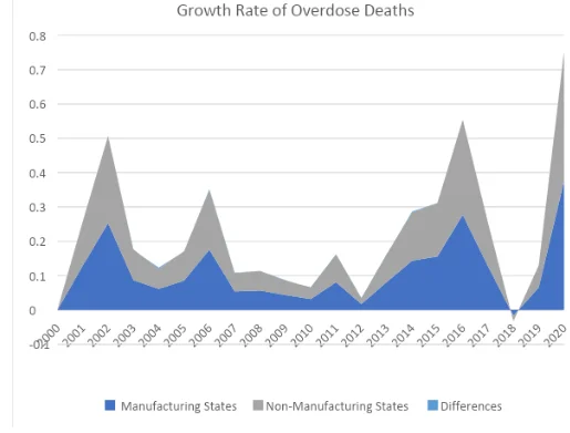
As we can see in Table 7, the differences between two types of states are really low.