OLS regression homework solution

Here, we have performed OLS regression using STATA and analyzed the results of income usage.

The data file cons.dta contains quarterly data on the log of real personal disposable income (Y) and the log of real personal consumption expenditure (C) for the US economy over the period 1960:1 to 2009:4.

a. For each series, decide whether it has a unit root or not. Use a formal test.

b. Regardless of the result in part a, assume now that both series have unit-roots. Estimate the simple consumption function (log consumption is a function of log income). What is the implication of the non-stationarity of the series for the results of the regression?

c. Now estimate a DL version of the function, i.e. with lags of income. Use OLS and HAC corrected standard errors.

d. Explain in words what the economic implications of the coefficients are.

e. Calculate the long-run marginal effect of log income on log consumption. Test the hypothesis that this is equal to 1.

f. In your opinion, does the model meet the requirements of the DL model in terms of the homogeneity of the regressors? Justify your answer.

a). Formal test for unit root

H_0:β=0 versus H_1:β>0

α=0.05

Test Statistic

DF=β ̂/(SEβ ̂ )

Decision Rule:

Reject H_0, if accept otherwise.

Output from Stata

For Income

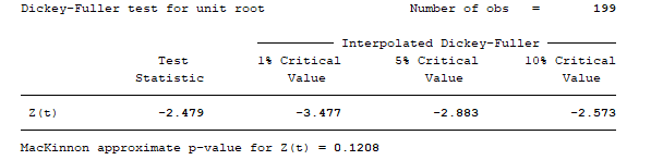
The MacKinnon p-value of 0.1208 implies that we do not have enough evidence to reject the null hypothesis of unit root at 0.05 level of significance and this implies that the Income is a non-stationary series.

For Consumption expenditure

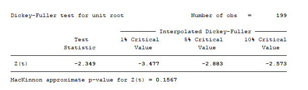
The MacKinnon p-value of 0.1567 implies that we do not have enough evidence to reject the null hypothesis of unit root at 0.05 level of significance and this implies that the consumption expenditure is a non-stationary series.

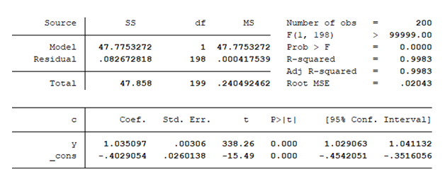
b) Regression output from Stata for marginal propensity to consume

The implication of non-stationarity of the series for the results of the regression is that the results will be misleading and biased in small samples.

c).

d). From the Stata, output, we can see that a unit increase in the logarithm of income level cause the consumption expenditure to go up by 1.035.

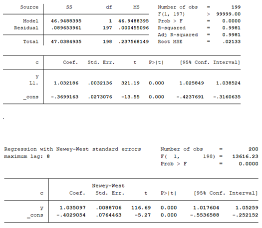
e). The long run marginal effect of log income on log consumption

H_0:mfx=1 versus H_1:mfx≠0

α=0.05

Test Statistic

mfx=df/dx

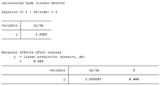
from the Stata output above, the long run marginal effect of log income on log consumption was computed as 1.035≈1.

Question 2

The file “rugby etc.dta” contains data on average tries per game in 6 nations rugby and the level of the NASDAQ stock market. Run a regression of tries on the NASDAQ and explain why 6 nations tries appears to cause the NASDAQ to move up! Explain how you would fix this problem and estimate a better model of the relationship.

Solution 2

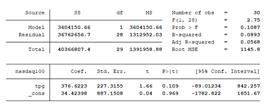
From the Stata output above, a unit increase in the average tries of the selected six games causes the stock price of NASDAQ to go up by 376.6223 and this could be attributed to the psychological impact of sports loss or win on investor. Sports win could positively trigger investor who can in turn induces others into following his actions and invariantly leading to an increase in the stock prices.

A more suitable approach would be to incorporate other market factors that can influence the performance of stock market into the model since sports result is only one of many triggers that can affect stock performance.

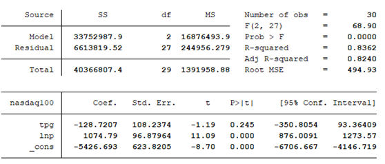
In the model outputted above, we incorporated the variable lnp into the regression model and we can easily see that inculcating lnp into the model reversed the positive relationship between NASDAQ prices and sports result, and this implies that to evaluate the impact of sports on stock performance, other relevant explanatory variables should be included in the model so as to efficiently analyze the impact of sports on stock prices.