Performing Normal Distribution
Here, we will use Minitab to carry out the normal distribution. Normal probabilities are calculated and the results are provided. Graphs are also used to show the standard limit theorem.
Questions
Part 1 – Calculating binomial probabilities
A company assembles paving machines. Periodically, samples of parts are collected and tested for quality control. If a part fails a specific test, it is assigned a ‘0’ and labeled defective. If apart passes the test, it is assigned a ‘1’ and then used in the assembly process. Use theAssembler data for Part 1.
1) Explain what distribution the defects follow and why specifically you know this
2) Use Minitab to calculate the probability of a defect, using the Assembler data.
Include your Minitab output
3) Model the defects and find the probability of no more than 14 defects
a) GraphàProbability Distribution Plot à View Probability
b) Distribution: (Use your answer from 1))
• Number of Trials: 80
• Event Probability: (Use your answer from 2))
c) Shade the area which is no more than 14 failed parts
• Windows: Shaded Area à X ValueàLeft Tail à X Value: 14
• Mac: OptionsàA specified X valueàLeft TailàX Value: 14
d) Include the Graph here
4) Based on your results and simulation, if you made 80 parts for a client, would they be likely to get more than 14 defective parts? Would you feel confident assuring your client that there will be less than 14 defects? Explain why
5) Estimate (do not calculate), based on your graph in 3) what the probability of 15-25 defects would be. Explain and justify your answer.
Part 2 – Calculating Normal probabilities
The average adult should be around 167.6 cm tall with a standard deviation of 9.3cm.
Assume height is normally distributed.
6) Use Minitab to determine the probability of being your height or taller. Show your Minitab output.
a) Use Calcà Probability Distributions à Normal…
b) Use the average adult for mean and standard deviation.
c) Use your height for Input Constant
d) Include the Output
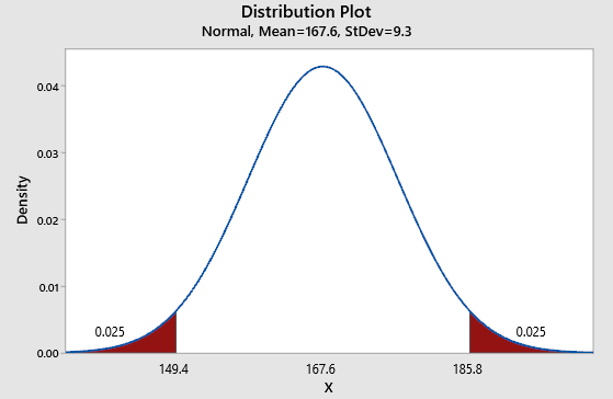
7) Using Minitab to determine the interval, centered on the mean, which contains 95% of adults. Show your Minitab output.
a) Graphs à Probability Distribution Plot à View Probability.
b) Use the average adult for mean and standard deviation.
c) Shaded Region à Both Tails. With the probability of 0.05
d) Include the Graph
Minitab Lab 2: Normal Distribution
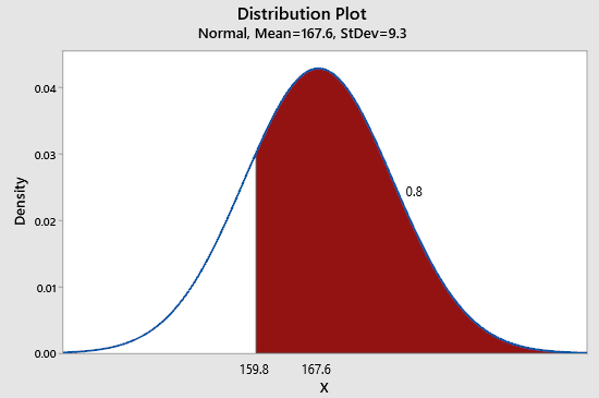
8) Use Minitab to determine the height that 80% of adults are taller than. Show your Minitab output.
a) Use either method from a) or b)
b) Include the Graph
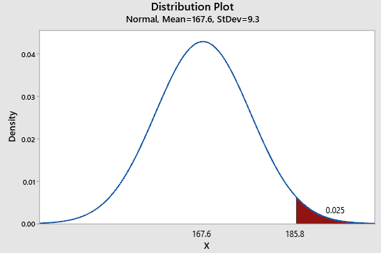
9) Based on the Empirical rule you know 2.5% of people are taller than what height? UseMiniTab to prove/illustrate this (Include the Graph)
Part 3 – Simulate the effects of the Central Limit theorem
Simulate a sampling distribution of the mean from a non-normal distribution. Open a blankMinitab worksheet to use for all the questions in this part.
10) Follow the instructions below to generate 200 rows of simulated random data using an exponential distribution, with λ=1.4. Store the data in columns C1 – C40.
Minitab Commands
i. Calc> Random Data > Exponential (Mac: Select Exponential from the
Random Data window)
ii. Number of rows to generate: 200
iii. Store in columns: C1-C40
iv. Scale: 1.4
v. Threshold: 0.0
Label column C40 as n=1. Label column C41 as n=6. Label column C42 as n=20. Label column C43 as n=40. See below.
Use row statistics to generate means from this data for different sample sizes (1,6,20,40).
b) For a sample of size 1, use the data in column C40 (labeled n=1).
c) Follow the instructions below for the remaining sample sizes (6, 20, and 40).
a. Calcà Row Statistics
b. Statistic: Mean
c. Input variables: C1-C6 (for sample size n=6)
d. Store result in C41
d) To generate means from samples of size 20repeat step b) and use input variables C1 –C20 and store in C42.
e) To generate samples of size 40 repeat step b)and use input variables C1 – C40 and store inC43.
f) Select Data à Worksheet Information. OK
g) Include the output
Minitab Lab 2: Normal Distribution
11) Create histograms of the distributions
a) Graph à Histogram
• Mac: Multiple Y-VariablesàDisplayed Separately
• Windows: Simple. Ok
- Multiple Graphs: In separate Panels of the same graph
b) Add variables C40-C43. OK
c) Include the Graph
12) What is the shape of each graph? (refer to its sample size in your explanation) What do you see as the sample size increases?
13) Calculate the mean and standard deviation for columns C40 – C43 and copy the values in this table and complete this table.
Column Mean Standard Deviation Theoretical SE
C40 Same
C41
C42
C43
14) Using the standard deviation from C40, a sample size of n=1
a) Calculate the theoretical standard deviation of the sampling distribution (Standard Error)for C41-C43, based on the formula and equation for standard error.
b) Add them to the table, and show your full calculations here. (Insert Equation)
15) Do the theoretical values match the simulation? (Within a small variation)
16) Create Probability Plots for each column C40-C43, in separate panels on the same graph
a) GraphàProbability Plot
• Mac: Multiple Y-VariablesàDisplayed Separately
• Windows: Simple. Ok
- Multiple Graphs: In separate Panels of the same graph
b) Add variables C40-C43. OK
c) Include the Graph
17) What happens to the shape of the distribution of the data as the sample size increases?
Explain
18) Compare the values in the table and probability plots and describe what happens to the mean as the sample size increases. Does this match theory?
19) Compare the values in the table and probability plots and describe what happens to the standard deviation as the sample size increases. Does this match theory?
Solution:
Part 1 – Calculating binomial probabilities
1) The distribution of defects follows binomial (1, p) distribution (known as Bernoulli). This is because each sample parts are independent, and the outcome can only be 1 or 0.
2) The probability of defects = 1 – 0.879 = 0.121
Statistics
Total
Variable Count Mean StDev Sum
Defects 124 0.8790 0.3274 109.0000
3)
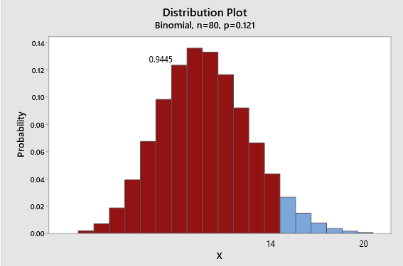
4) The probability that client will have no more than 14 failures is 0.9445. They can be 94.45% confident that there would be less than 14 defects.
5) The probabilities will be 1 – 0.9445 = 0.0555
The probability beyond 25 will be too small seeing the graph. So remaining probability would be between 15 and 25.
Part 2 – Calculating Normal probabilities
6) The probability of being my height (170cm) or taller is 1-0.6018 = 0.3982
Normal with mean = 167.6 and standard deviation = 9.3
x P( X ≤ x)
170 0.601821
7) The interval is [149.4, 185.8].
8) The height is 159.8
9) Only 2.5% of people are taller than 185.8cm.
Part 3 – Simulate the effects of the Central Limit theorem
10) Output
Columns
Column Count Name
C1 200
C2 200
C3 200
C4 200
C5 200
C6 200
C7 200
C8 200
C9 200
C10 200
C11 200
C12 200
C13 200
C14 200
C15 200
C16 200
C17 200
C18 200
C19 200
C20 200
C21 200
C22 200
C23 200
C24 200
C25 200
C26 200
C27 200
C28 200
C29 200
C30 200
C31 200
C32 200
C33 200
C34 200
C35 200
C36 200
C37 200
C38 200
C39 200
C40 200 n=1
C41 200 n=6
C42 200 n=20
C43 200 n=40
11) Graph
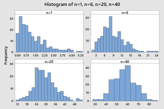
12) Shape for n=1 is skewed right. Shape for n=6 is also skewed right but less skewed. Shape for n=20 is almost symmetric bell shaped. Shape for n=40 is symmetric bell shaped.
We see that as sample size increases, the shape of the distribution approaches to symmetrical bell-shaped.
13)
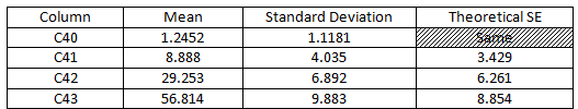
14) The standard error for the C41-C43 can be given by σ_n=√n×σ
σ_6=√6×σ=√6×1.4=3.429
σ_20=√20×σ=√20×1.4=6.261
σ_40=√40×σ=√40×1.4=8.854
15) The theoretical values are close to simulation with small variations.
16)
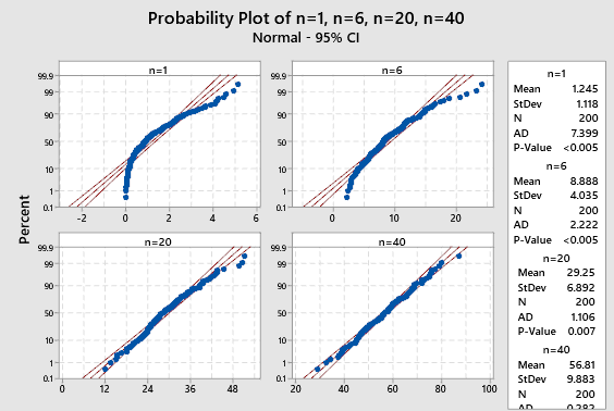
17) The shape of distribution approaches the normal distribution as n increases. The n=1 and n=6 are not straight lines in a normal P-P plot. But n=20 is closer to the straight line and n=40 is very close to a straight line.
18) The mean increases linearly as the sample size increases. This matches the theory as
μ_N=N×μ
19) The standard deviation increases by a factor of √n as the sample size (n) increases. The result matches the theory.
σ_N=√N×σ