Using means and standard deviation to determine results
In this task, we use both means and standard deviation to determine the amount of weight loss since the start of the exercise. We will also apply both multiple linear regression and multiple logistic regression to see the relationship between weight loss and some personal characteristics.
Question
Evaluate if there is a relationship (predict) between the personal characteristics and the screening tools with weight loss. Prepare a short description of what was done and what you found. IV=independent variable, DV= dependent variable
Conduct a multiple linear regression to predict satisfaction using all of the personal characteristics and perception variables (if appropriate).
Follow the guide in Module 9 on how to conduct this analysis and include in your description what you did such as the following:
a. Define the hypothesis
b. Describe each variable using appropriate descriptive statistics; no need to recode anything but make sure dummy coding is correct; create a ‘table1-remember analysis exercise 1’for this step
c. Run bivariate associations (why? need IV by each IV to check for _________)
d. Run the full model (DV and multiple IVs ) –show evidence that you checked assumptions, etc (for this exercise it is ok to enter the selected IVs all at once in one ‘block’)
e. Summarize the above (a-d) and the results in your OWN words
f. Include IS raw output view or the Excel output.
Solution
a. Hypothesis
Null hypothesis: there is no relationship between the dependent variable (Islost) and the independent variable (sex, age, diet, exercise, confid, sedentary)
Alternative hypothesis: there is at least a relationship between the dependent (Islost) and the independent variable (sex, age, diet, exercise, confid, sedentary)
H_0: μ_1=μ_2=μ_3=μ_4=μ_5=μ_6
H_a: μ_1≠μ_2≠μ_3≠μ_4≠μ_5≠μ_6
b. Descriptive statistics
| n | Mean | Median | Standard Deviation | |
| Age | 51 | 26.94 | 23 | 8.09 |
| Excercise | 51 | 39.59 | 39 | 5.49 |
| Confid | 51 | 17.78 | 17 | 3.37 |
| Sedentary | 51 | 114.39 | 114 | 4.40 |
| lbs lost | 51 | 24.43 | 24 | 5.07 |
| sex | 51 | Female (57%) | Male (43%) | |
| diet | 51 | Yes (63%) | No (37%) |
The table above shows the descriptive statistics of the weighted dataset. 57% of the total participants are female while 43% of the participant are male. 63% of the participant have diet adherence while 37% do not have diet adherence. The average age of participants was 26.96 years (SD = 8.09). The mean and standard deviation of minutes exercising per day is (39.59, 5.49), confidence in success (M = 17.78, SD = 3.37) respectively, minutes inactive per day (M = 114.39, 4.40), pounds lost since the start of the program (24.43, 5.07).
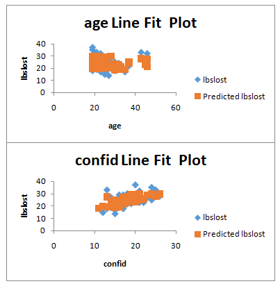
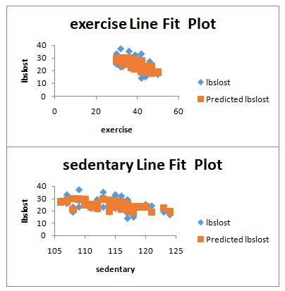
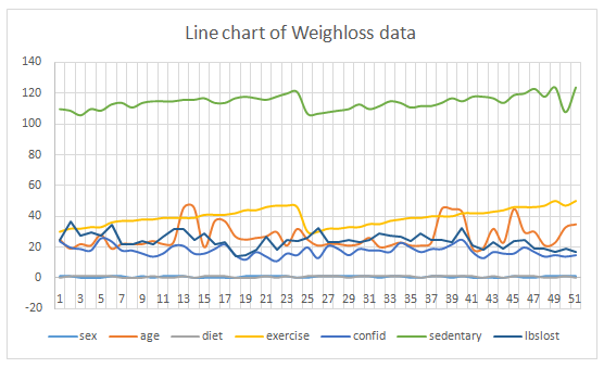
c. The bivariate association graph above shows the bivariate relationship between the dependent variable and the independent variables. The dependent variable is weight loss while the independent variables are age, exercise, sedentary, and confid.
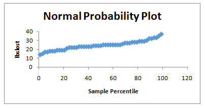
d. The following are the assumption of multiple linear regression which is illustrated from the graphs below;
- There exists a linear relationship between the dependent and independent variables
- The independent variables are not highly correlated with each other
- The variance of the residuals is constant
- Independence of observation
- Multivariate normality i.e. it follows a normal distribution
e. Multiple regression (OLS) was used to estimate the ability sex, age, diet, exercise, confidence in success, minutes inactive per day, in predicting weight loss. Forty-five percent of the variance surrounding weight loss was explained by sex, age, diet, exercise, confidence in success, minutes inactive per day weight (R2 = 0.4567). Overall, the model was statistically significant weight loss (F = 6.1667, p = 0.000). Sex, Age, Exercise, Confidence in success, and Minutes inactive per day was not statistically significant in the model (p > 0.05); whereas diet was statistically significant (t = 2.096, p = 0.04). For every one cm increase in head circumference, motor coordination scores increased by 0.65 points (beta = 0.65). Males were also found to score higher than females. Males scores were .35 points higher (beta=.35, p=.04).
f.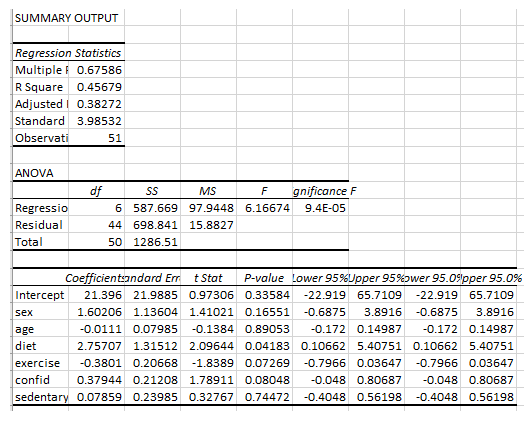
Part B. Multiple logistic regression
Question
Task: Now we would like to see if we can find a relationship (predict) between weight loss and some of the personal characteristics and the chance of recommending the clinic to others.Prepare a short description including the following information:
1. Is running a multiple logistic regression appropriate for this task? Explain why it is or is not appropriate.
2. Define the hypotheses
3. How many and what percent of patients indicated they would recommend the clinic?
4. You do not need to run logistic regression in EXEL or IS. Use the output below to write a summary of the relationship.
Solution
1. Is running a multiple logistic regression appropriate for this task? Explain why it is or is not appropriate.
Answer: Yes, this is because the outcome or target variable is binary (yes or no) and since the number of observations is greater than the number of features in the datasets, there is no room for overfitting in the model.
2. Define the hypotheses
Ans: H_o: There is a relationship between weight loss and some of the personal characteristics and the chance of recommending the clinic to others.
i.e. H_o=μ_0= μ_1…=μ_n
H_1: There is a relationship between weight loss and some of the personal characteristics and the chance of recommending the clinic to others.
i.e. H_1≠μ_0≠ μ_1…〖≠μ〗_n
3. How many and what percent of patients indicated they would recommend the clinic?
Ans: 25 (Twenty-five) patients and 49 % of patients indicated that they would recommend the clinic.
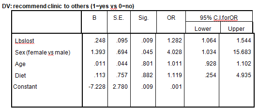
4. Logistic multiple regression was used to estimate the ability of Age, Sex, Lbslost, and Diet in predicting if the patients will recommend the clinic (yes) or not (No). Age and Diet were not statistically significant in the model (p > 0.05). A significant association was found between variables: Lbslost, Sex, and Patients recommending the Clinic and there’s no significant relationship between Age, Diet, and Patients recommending the Clinic. An increase in sex of the patients will increase the odds of recommending the clinics by four-fold (Odds ratio= 4.03, 95% confidence interval= 1.034, 15.68, p<.001), an increase in Lbslost of the patients will increase the odds of recommending the Clinic by almost two-fold (Odds ratio= 1.28, 95% confidence interval= 1.064, 1.544, p<.001) and an increase in Age (Odds ratio= 1.011, 95% confidence interval= 0.928, 1.102, p<.001) and Diet (Odds ratio= 1.119, 95% confidence interval= 0.254, 4.935, p<.001) of the patients will increase the odds of recommending the Clinic by one fold respectively.
Part C. Sensitivity & Specificity
Question
Recall that our survey used a self-report measure of diet adherence. We want to assess if the results are valid and accurate by comparing the self-report with a gold standard (stool sample detecting microbiome and should see only small amounts of fats and sugars, etc). We identify 15 true positives out of the 32 clients who self-identified as being diet adherent and 18 true negatives.
1. Fill in the following table
| Gold standard positive | Gold standard negative | Total | |
| Self-report + adherence | |||
| Self-reports non-adherence | |||
| Total |
2. Calculate the sensitivity of the self-report measure.
3. Calculate the specificity of the self-report measure.
4. What does this mean—was our self-report of diet adherence a good measure? What does having a good or poor measure mean when exploring relationships, how do you think about it when applying these kinds of evidence-based findings?
Solution
1. Fill in the following table
| Gold standard positive | Gold standard negative | Total | |
| Self-report + adherence | 15 | 17 | 32 |
| Self-reports non-adherence | 14 | 18 | 32 |
| Total | 29 | 35 | 64 |
2. Calculate the sensitivity of the self-report measure.
Sensitivity = 15/32 = 0.46875
3. Calculate the specificity of the self-report measure.
Specificity = 18/32 = 0.5625
4. What does this mean—was our self-report of diet adherence a good measure? What does having a good or poor measure mean when exploring relationships, how do you think about it when applying these kinds of evidence-based findings?
Since both sensitivity and specificity have average values, it does not indicate a good measure.
Part D. Run Chart
1) Did the proportion of women administered RhoGam vaccination change—what was the mean before and after the program change?
From the data provided, I notice that the proportion of women administered RhoGam vaccination change, the mean before program change is 51.89 while the mean after program change is 51.33
2) Did all the changes that were made lead to improvements?
The changes that were led do not lead to much improvement based on the data analyzed using the run chart.
3) What data would you want to start collecting to determine other steps for quality improvement in these patients?
In other to determine other steps for quality improvement in the patients, I will suggest that data can be collected on the average glucose intake, percentage of time in hypoglycemic ranges, and percentage of time in hyperglycemic range.