Homework Problem Description:
This STATA homework aims to analyze and present the results of a study on the impact of micro-loans and free group interventions on hemoglobin (Hb) levels. The analysis includes baseline characteristics, intent-to-treat (ITT) effects on endline Hb levels, difference-in-difference (Diff-in-Diff) estimation, and the assessment of heterogeneous effects with Diff-in-Diff estimation. Here's the structured presentation of the solution:
Solution
1. Baseline characteristics
| variable | mean | sd |
|---|---|---|
| control | 10.907 | 1.856 |
| micro-loans | 10.956 | 1.802 |
| free group | 10.696 | 1.906 |
The result showed that the Hb levels in the microloans group is the highest at baseline (M=10.956, SD=1.802) while the Hb level of the free group is the lowest (M=10.696, SD=1.906). the control group lie in-between (M=10.907, SD=1.856)
B
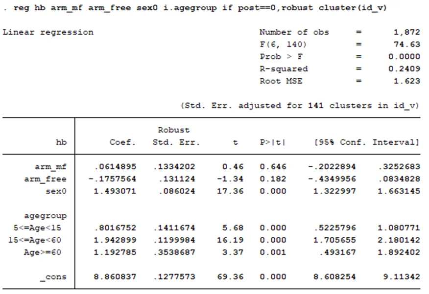
The result showed that the estimated coefficient of arm_mf is not significant (p>.05) which suggests there is no statistically significant difference in the baseline Hb level between the micro-loans arm and the control after controlling for gender and age group. Similarly, the estimated coefficient of arm_free is not significant (p>.05) which suggests there is no statistically significant difference in the baseline Hb level between the free arm and the control after controlling for gender and age group.
2. Intent to Treat effect on endline Hb levels
A
The result showed that the Hb levels in the microloans group is the highest at follow-up (M=11.28, SD=1.80) while the Hb level of the free group is the lowest (M=11.177, SD=1.8). the control group lie in-between (M=11.19, SD=1.76)
| variable | mean | sd |
|---|---|---|
| control | 11.177 | 1.798 |
| micro-loans | 11.279 | 1.802 |
| free group | 11.190 | 1.763 |
B
| (1) | (2) | |
|---|---|---|
| hb | hb | |
| arm_mf | 0.10 | 0.10 |
| (0.32) | (0.47) | |
| arm_free | 0.01 | 0.01 |
| (0.90) | (0.93) | |
| _cons | 11.18*** | 11.18*** |
| (0.00) | (0.00) | |
| N | 1874 | 1874 |
p-values in parentheses
*p< 0.05, **p< 0.01, ***p< 0.001
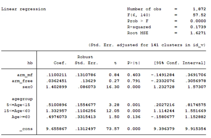
The result showed that the estimated coefficient of arm_mf is not significant (p>.05) for both clustered and unclustered model which suggests there is no statistically significant difference in the average follow-up Hb level between micro-loans arm and the control after controlling for gender and age group. Similarly, the estimated coefficient of arm_free is not significant for both clustered and unclustered model (p>.05) which suggests there is no statistically significant difference in the average follow-up Hb level between the free arm and the control after controlling for gender and age group.
C
The result above showed that the intention to treat for the micro-loans group is 0.11 after controlling for age and gender but the ITT is not statistically significant (p>.05). Similarly, the intention to treat for the micro-loans group is 0.04 after controlling for age and gender but the ITT is not statistically significant (p>.05).
D
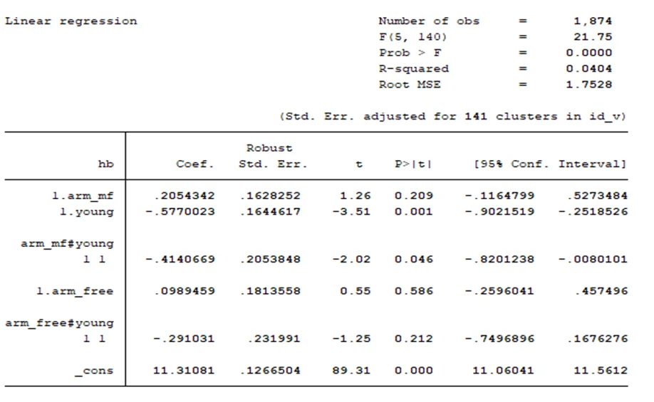
The result presented above showed that the interaction between micro-loans group and the binomial variable representing whether the respondent is 10 years or below or not is slightly significant (p=.046). Thus, there is slight evidence of heterogeneous effect of the micro-loans for those 10 years old or less as they will have lower Hb than their counterpart who are also micro-loans arm but are older than 10 years. Conversely, the interaction between free arms and the binomial variable representing whether the respondent is 10 years or below or not is not significant (p=.2). Thus, there is no evidence of heterogeneous effect of the free arms for those 10 years old or less.
3. Diff-in-diff estimation
A
The regression equation to estimate diff-in-diff is given as
Hb=α_0+β_1 arm_mf+β_2 arm_free+β_3 post+δ_1 arm_mf×post〖+δ〗_2 arm_free×post+α_1 age+α_2 gender+ϵ
From the equation above, the two treatment groups are arm_mf and arm_free, the time variable is post denoting post treatment and pre treatment. age and gender are control variables. The diff-in-diff estimate is δ_1for the arm_mf group and δ_2 for arm_free group.
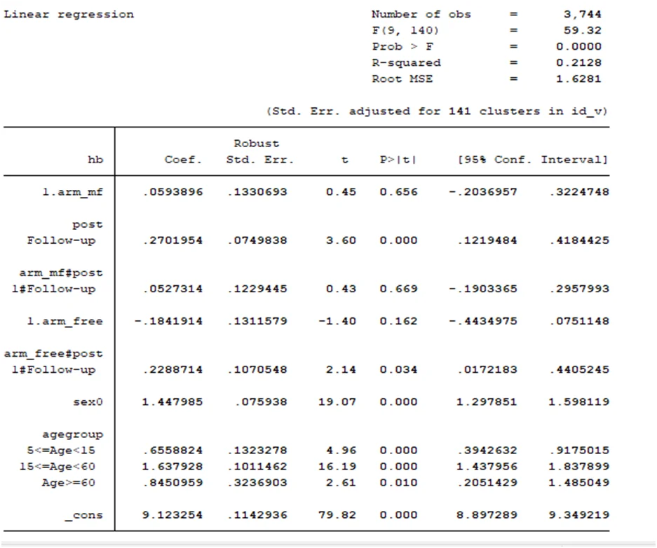
The result of the model is presented below.
From the result, the diff-in-diff estimate for micro-loan group is 0.052 but not significant (p=.67) while the diff-in-diff estimate for free arm is 0.23 and is significant (p=.03).
B
The findings from diff-in-diff estimate is opposite of what is found for ITT. In ITT, the micro-loan effect is significant but the free-arm is not significant. In contrary, the diff-in-diff estimate the effect for free-arm is significant while the effect for micro-loan is not significant.
4. Heterogeneous effects with diff-in-diff estimation
A
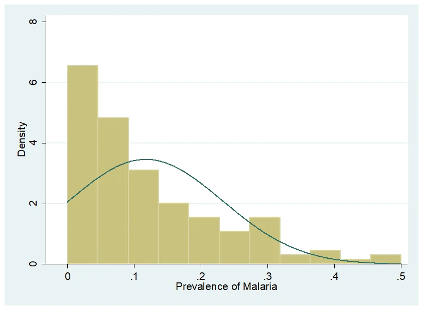
The histogram for malaria prevalence at village level is shown above. It is observed from the plot that distribution of malaria prevalence is skewed.
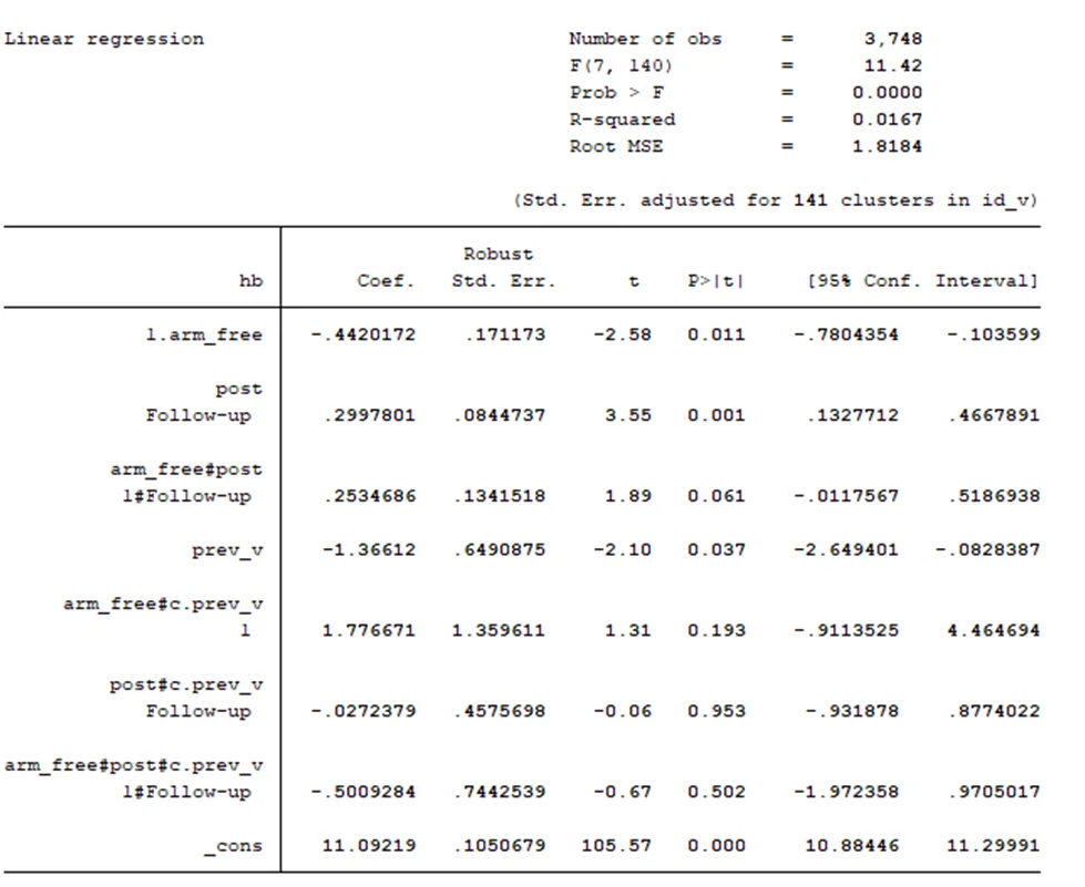
B
The regression model to measure the heterogeneity of treatment effects by the village-level baseline prevalence of malaria is presented below. to achieve this, an interaction of free arm indicator, time and malaria prevalence was added to diff-in-diff model. This interaction is not significant (p=.5) which suggests that there is no significant heterogeneity of treatment effects by the village-level baseline prevalence of malaria and the treatment effect is the same no matter the prevalence of malaria.