Assignment instructions
Produce plots to explore the relationship, or lack thereof, between your response variable, and each of these potential predictors, choosing appropriate plots for the types of variables analyzed. Describe any relationships that arise.
Model selection
Build a linear model to predict evaporation (in mm) on a given day in Melbourne, using all of the predictors listed in the Bivariate summaries paragraph above. Also consider an intersection term between a month and 9 am relative humidity, to determine whether humidity has a different effect in different months. Your model should include all predictors with a significant effect on evaporation, and no predictors that are not significant. In order to do this, produce your model according to the following process:
1. Fit a model containing all the possible predictors.
2. Determine the p-value for inclusion of each predictor: i. P-values for quantitative variables can be determined using the linear model summary.
ii. P-values for categorical variables, or intersections containing categorical variables, can be determined using an ANOVA.
3. Remove the predictor with the highest p-value for inclusion, unless all remaining predictors are significant at the 5% level.
4. Update your model to include only the remaining predictors.
5. Repeat Steps 2-4 until only significant predictors remain.
Interpret the coefficients of your model in context. This includes the intercept, and the coefficients relating to each predictor. Your interpretation should be done in a manner that can be interpreted by your client.
For categorical predictors, you do not need to explain all coefficients but provide an overview of how the model operates in relation to these terms, with an example of one of the coefficients.
Model diagnostics
Test all of the assumptions of your linear model.
Prediction
MWC is interested both in the general application of your model, and in some particular extreme scenarios that it envisages. They thus seek your predictions for the amount of evaporation, in mm, for days of the following character:
• February 29, 2020, if this day has a minimum temperature of 13.8 degrees and reaches a maximum of 23.2 degrees, and has 74% humidity at 9am.
• December 25, 2020, if this day has a minimum temperature of 16.4 degrees and reaches a maximum of 31.9 degrees, and has 57% humidity at 9am.
• January 13, 2020, if this day has a minimum temperature of 26.5 degrees and reaches a maximum of 44.3 degrees, and has 35% humidity at 9am.
• July 6, 2020, if this day has a minimum temperature of 6.8 degrees and reaches a maximum of 10.6 degrees, and has 76% humidity at 9am.
Provide a table containing appropriate intervals for making forecasts on these particular days, and explain the intervals in context. Compare and contrast potential amounts of evaporation on different days.
If there is more than 10mm of evaporation at MWC’s Cardinia Reservoir, the corporation takes temporary measures to ensure a continuous supply of water, including transferring water from its Silvan Reservoir upstream:
• For which of the predicted days can we say with 95% confidence that this will occur?
• For which of the predicted days can we say with 95% confidence that this will not occur?
Assignment Solution
Assignment 2
Executive Summary
The analysis of Melbourne’s weather observations data shows the relationship between the evaporation on a given day with attributes like a day of the month, month, the maximum and minimum temperature for 24 hours to 9AM, and relative humidity at 9 AM. The analysis of the data shows that Minimum temperature, Month, relative humidity, and interaction between relative humidity and month were found to be significantly affecting the evaporation for the day. The statistical model was tested to be effective for predicting evaporation using these attributes. However, the day of the month did not show any relationship with the evaporation which was expected all along. The analysis shows that evaporation is high in the summer season and low in the winter season with peaks being around January and lowest around May-June.
Methods
The analysis of Melbourne’s weather observations data shows the relationship between the evaporation on a given day with attributes like a day of the month, month, the maximum and minimum temperature for 24 hours to 9AM, and relative humidity at 9AM. R was used as the choice of statistical software for all purposes of computation in this work due to its vast capabilities. The incomplete data points which had NA’s in evaporation was removed in the start to have only the complete cases in the analysis.
Bivariate Summaries
The first step in analyzing the data is exploratory analysis. In next section of bivariate summaries, relationship between the response variable, evaporate, and all the predictor variables have been explored individually to get a sense of the direction of the analysis.
Month
The month variable represents the calendar month of the date where the observation was made. The month variable is expected to have a significant impact on evaporation as different months can have different weather leading to different levels of evaporation. A boxplot was used to look at the difference in evaporation by month.
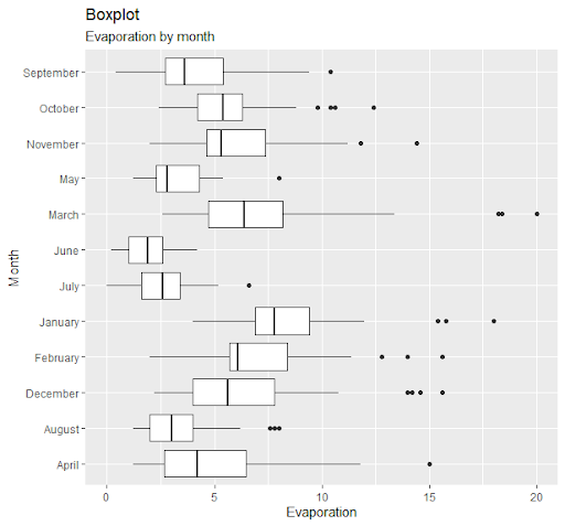
The plot resonates with the expectations that there would be a quite significant difference in levels of evaporation for different months. From the plot, it can be noted that the May-Aug period shows less evaporation and Dec-Mar shows higher evaporation levels.
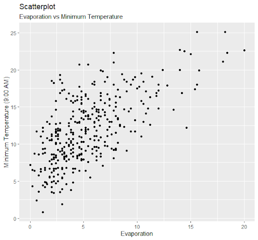
Figure 4:Scatterplot between evaporation and maximum temperature. The plot shows an increasing relationship between evaporation and maximum temperature.
As expected, the scatterplot shows strong relationship between evaporation and maximum temperature.
Relative humidity (9:00 AM)
Relative humidity variable records the Relative humidity at 9 am. It is also expected to have strong effect on the evaporation as higher humidity should lead to low evaporation as water content on air will have a saturation point. Scatterplot was used to study the significance of the relationship with evaporation on x-axis.
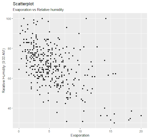 Figure 5: Scatterplot between evaporation and relative humidity. It shows a negative relationship between the two
As expected, we do see a strong visible decreasing relationship between evaporation and relative humidity.
Model Selection
• The first model was built with evaporation as the dependent variable and day, month, minimum, and maximum temperature, relative humidity, and interaction between month and relative humidity as predictors. The model had multiple R2 of 0.6383. In terms of significance of the variables, day (p=0.74) and maximum temperature (p=0.70) was found to be statistically insignificant. On this step, day variable was removed.
• Model was fitted again with all the previous predictors excluding day variable. This time, only maximum temperature (p=0.71) was found to be statistically insignificant. Hence, maximum temperature was dropped in the next model fit.
• Third model was fitted with evaporation as dependent variable and month, minimum temperature, relative humidity, and interaction between month and relative humidity as predictors. In this model, all variables were found to be statistically significant.
The final model which had all the variables statistically significant was model 3 with month (p<0.001), minimum temperature (p<0.001), relative humidity (p<0.001), and interaction between month and relative humidity (p<0.001).
Expectation vs reality?
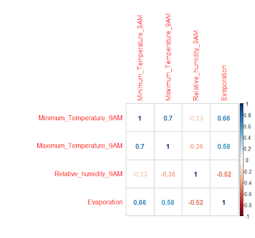
These terms differ from what we expected in bivariate summaries where we expected maximum temperature to be impactful but as it turned out, it was not statistically significant. This might have happened because of the multicollinearity. Since we expect high correlation between minimum and maximum temperature, essentially hot days have both minimum and maximum temperature high and vice versa, the information available in maximum temperature is captured in the variable minimum temperature. The correlation between minimum and maximum temperature was 0.70 which is quite high. Hence, even though maximum temperature would have been significant standalone, it was not significant in presence of minimum temperature.
However, all the other terms which was expected to be significant in the bivariate summaries are indeed significant.
Model Diagnostics
The linear model implemented in this work comes with few assumptions which have been outlined below and tested in the appendix of the report.
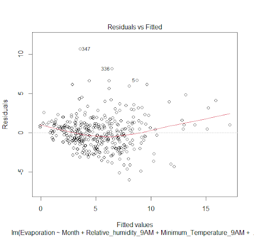
1. Homoscedasticity: The variance of residual is the same for any value of X. This was tested through scatterplot of fitted vs residuals.
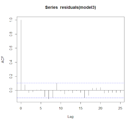
2. Independence: Observations are independent of each other. This assumption was tested using ACF and PACF of the residuals.
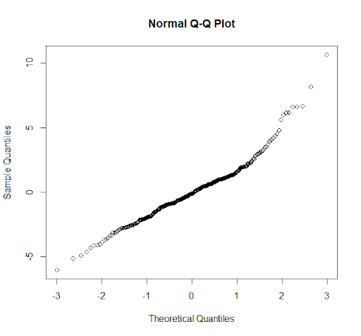
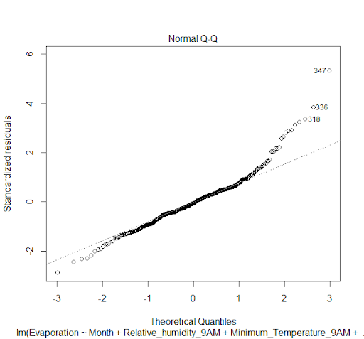
3. Normality: Residuals are normally distributed. This was tested through normal Q-Q plot.
4. No multicollinearity: The independent variables should not be correlated. This was tested using correlation matrix.
For assessment, readers are referred to the Appendix section of this report.
Result
Model Interpretations
The final model which was selected for the prediction in this work had evaporation as dependent variable and month, minimum temperature, relative humidity, and interaction between month and relative humidity as predictors. In R, the first category from alphabetical order was selected as reference for Month, hence April is the reference month variable and interaction term. The slopes and intercept of the models can be interpreted as below:
• Intercept (10.56) – The intercept represents the average evaporation value when the numeric variables are set to 0 and the categorical variable are set to reference categories. Here, if minimum temperature is 0, relative humidity is 0, and month is of April, then the average evaporation is estimated to be 10.56mm.
• Relative Humidity (-0.147) - Slope of relative humidity indicates that if all the other variables are kept same, the change in evaporation for each unit increase in relative humidity will be -0.147mm.
• Minimum Temperature (0.369) - Slope of minimum temperature indicates that if all the other variables are kept same, the change in evaporation for each unit increase in minimum temperature will be 0.369mm
• Month – The slopes in different categories of the month represents the average estimated change in evaporation compared to the month of April, if all the other variables are kept same. Hence, slope of June (-10.348) represents that if all the other variables are kept same, then the evaporation will decrease by 10.348mm, on an average, in June as compared to month of April.
• Interaction between Month and Relative Humidity – The slopes in these categories represent the change in evaporation per unit increase in relative humidity as compared to month of April at a given level of relative humidity, if all the other variables are kept same. Hence, slope of Aug in interaction terms (0.136) shows that evaporation will be 0.136*Relative Humidity higher than that in month of April at same relative humidity.
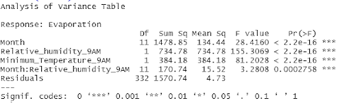
The ANOVA Table of the model shows the contribution of each variable towards explaining the variance of the data.
| 95% Prediction Interval | |
| Date Fitted | Lower Upper |
| February 29, 2020 5.506 | 1.089 9.923 |
| December 25, 2020 8.606 | 4.209 13.003 |
| January 13, 2020 14.872 | 10.105 19.640 |
| July 6, 2020 2.265 | -2.111 6.642 |
Model Diagnostics Assessment