Paired Samples T-Tests Assignments
INSTRUCTIONS: For this exam, you will design and test one of each of the listed hypothesis test types. This time, you are in the driver’s seat and will have to decide what research questions YOU want to answer, using the data that is provided for you! This dataset contains randomly generated data from 20 different demographic and college-test-related variables from 100 seniors attending different state universities in NJ.
For each test, you should do the following (you must show each numbered and lettered step below).
1. Create a research question that you can answer appropriately using the test and using the available data. Each variable contains labels that describe what was measured, and there are a variety of nominal and scale variables from which you can choose.
2. Identify the appropriate variables for your research questions, their measurement type, and their label(as this information appears in SPSS)
3. Compute descriptive statistics using Analyze →Descriptives →Explore command and copy your output table. You should also write a few sentence descriptions summarizing your variables.
4. Complete the following three steps of hypothesis testing
a. Step 1: Null/Alternative hypotheses
b. Step 2: Alpha level, degrees of freedom (if appropriate), one/two-tailed test type (if appropriate), other information as appropriate
c. Step 3: Appropriate test statistic/table, as a copied and pasted/screenshot of SPSS results
i. Post hoc tests if appropriate
d. Step 4: A full write up for step four, including:
i. A decision about the null hypothesis
ii. A written explanation about the results of the test, including means and standard deviations, and a final answer to your research question
iii. Proper APA style string, including effect size and confidence intervals, if appropriate.
Please conduct one of each of the following hypotheses tests:
1. Paired-Samples t-test
2. Independent Samples t-test
3. One-Way ANOVA
4. Correlation
5. Regression
6. Two-way Chi-Square
Solution:
Paired-Samples t-test
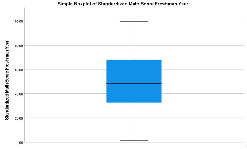
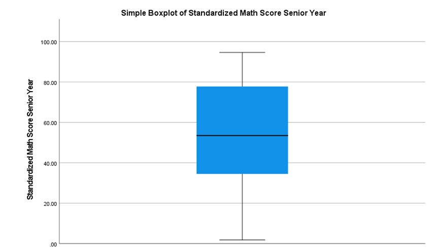
1. Is the mean standardized math score for freshman and senior year the same.
2. Variables used for this study are “MathScore_Freshman”, Measurement Type: Scale, and “MathScore_Senior”, Measurement Type: Scale.
3.
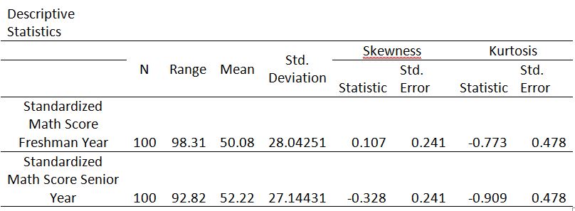
The mean standardized math score for Freshman was 98.31 whereas the Mean standardized math score for Senior Year was 98.31
4. Step 1. H0: μ_d=0
Ha: μ_d≠0
Step 2. α = .05
Step 3.
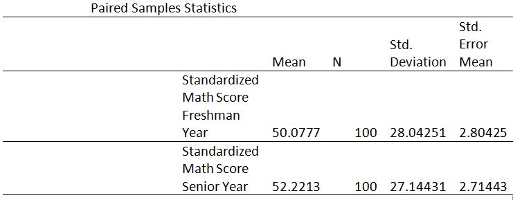
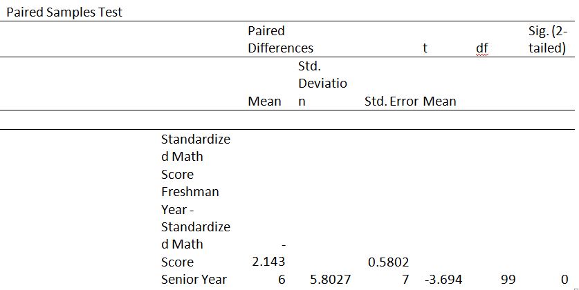
Step:4 Reject Null hypothesis, As the paired t-test showed that standardized math score for Freshman (M=50.8, SD=28.04)and standardized math score for Senior(M=52.22, SD=27.14) are significantly different at a significance level of 0.05.
Independent-Samples t-test
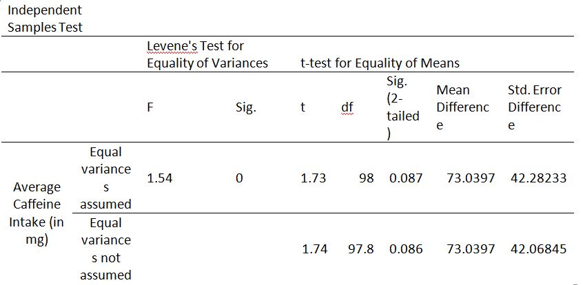
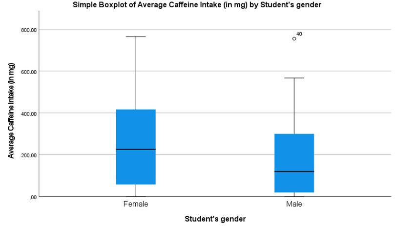
1. Is the average caffeine intake the same for males and females.
2. IV:” Gender”, Measurement Type: “Nominal”. DV: ”Avg_CaffeineIntake”, Measurement Type: “Scale”.
3.
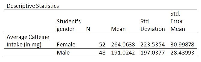
Mean caffeine intake by females is 264.0638 and by males is 191.0242 whereas their respective standard deviation is 223.5354 and 197.0377 respectively.
Step 1. H0: μ_males=μ_females
Ha: μ_males≠μ_females
Step 2. α = .05
Step 3.
Step 4.
Retain H0. Levene’s test showed that the variance was equal between the two genders, p = .316. There was not a significant difference in average caffeine intake by males (M = 191.02, SD= 197.04) and females(M=264.06,SD=223.54).T-statistics=1.74 and p-value=0.086(>0.05).
One-Way ANOVA
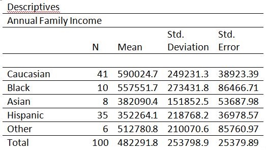
1. Is there a significant difference in family income of students belonging to different races.
2. IV: “Race.” Label: “Student's race.” Measurement Type: Nominal
DV: “FamilyIncome.” Label: “Annual Family Income.” Measurement Type: Scale
3.
4.
Step 1. H0: μ_1= μ_2= μ_3
Ha: Not all μ's are equal.
Step 2. α = .05
Step 3
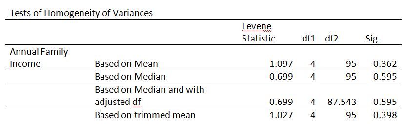
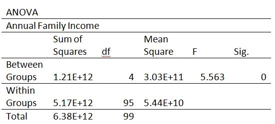
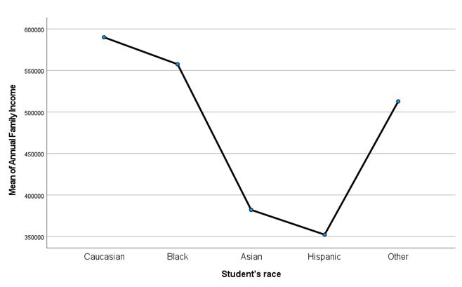
Step 4. Reject H0. Levene’s test showed that the variance was equal between the 5 groups, F(2, 97) = 1.097, p = .362. There was a significant difference in the average annual family salary of students of various races. Caucasian (M=590024.7,SD=249231.3), Black (M=557551.7,SD=273431.8), Asian (M=382090.4,SD=151852.5), Hispanic (M=352264.1,SD=218768.2), Other (M=512780.8,SD=210070.6). F (4,95)=5.563, p-value=0.0000.
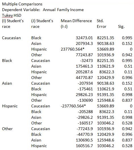
From the post hoc table, we can see that there is a significant difference in the average annual family income of the Caucasian and Hispanic students.
Correlation
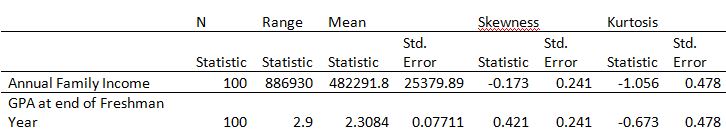
1. Is there any significant correlation between average family income and GPA at the end of the first year.
2. IV: “FamilyIncome.” Label: “Annual Family Income.” Measurement Type: Scale,
IV: “GPA_Freshman.” Label: “GPA at end of Freshman Year.” Measurement Type: Scale
3.
4.
Step 1. H0: ρ=0
Ha: correlationρ≠0
Step 2. α = .05
Step 3.
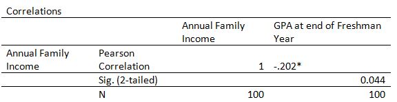
Reject H0:There is sufficient evidence that there is a significant correlation between Annual family income and GPA at the end of Freshman Year.
Regression
1. Is there any Linear relationship between FRESHMAN GPA and senior GPA.
2. IV: “GPA_Freshman.” Label: “GPA at end of Freshman Year.” Measurement Type: Scale
DV: “GPA_Senior.” Label: “Current Senior GPA.” Measurement Type: Scale.
3.
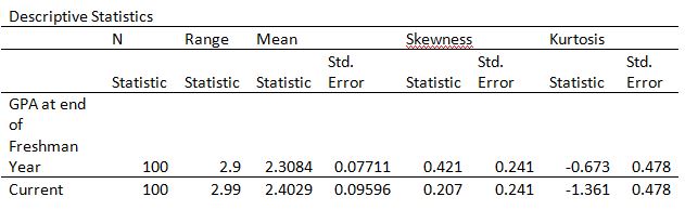
The average GPA at end of Freshman Year is 2.9 whereas the Average Current Senior GPA is 2.99.
4.
Step 1. H0: β=0
Ha: β≠0
Step 2. α = .05
Step 3.
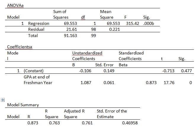
Reject H0: From the Anova table, we can see that model is predicting significantly better than just predicting the average value for all the responses. And GPA at end of Freshman Year(coefficient=1.087,sd=0.061,p-value=0.000).The value of R^2 is 0.873 this means 87.3% variance in senior GPA is explained by GPA at end of Freshman Year.
Two-way Chi-Square
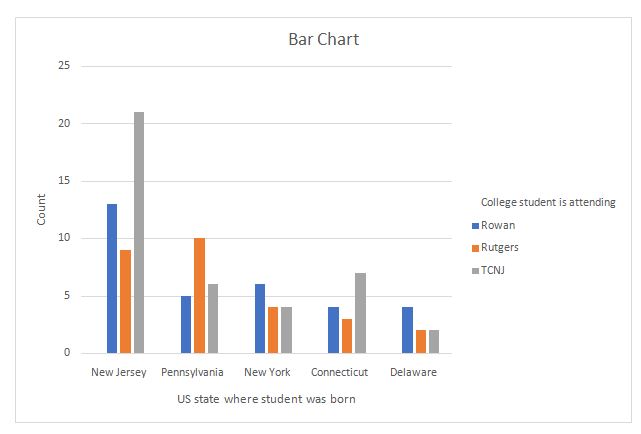
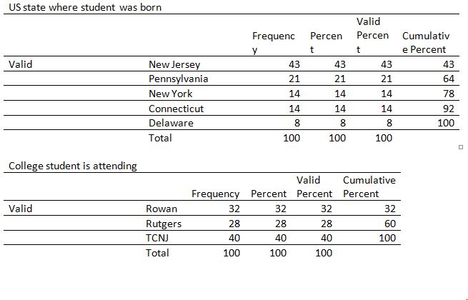
1. Is there any dependency between Birthplace and college?
2. IV: “BirthState.” Label: “US state where the student was born.” Measurement Type: Nominal
DV: “College.” Label: “College student is attending.” Measurement Type: Nominal.
4.
Step 1. H0: Birthplace and college of study are independent of each other
Ha: Birthplace and college of study are not independent of each other
Step 2. α = .05
Step 3.
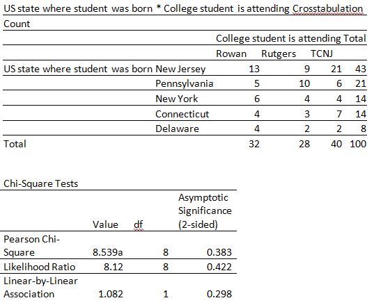
Retain Ho: We don’t have enough evidence to reject the null hypothesis and conclude that Birthplace and college of study are independent of each other.