Regression Models for Predicting House Prices and Response Relationships in R

Problem Description:

The R Programming homework focuses on analyzing a dataset to build and evaluate regression models for predicting house prices in different scenarios. It involves data transformations, regression coefficients, residual diagnostics, model comparison, and statistical inference. The goal is to understand the relationships between various variables and make predictions about house prices.

Solutions

Question 3

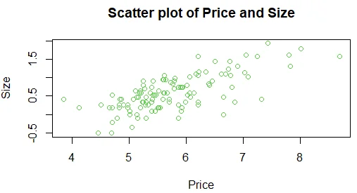
For this model to be better, a transformation of log-log works better, the resulting scatter plot is as shown in the figure below.

Question 4

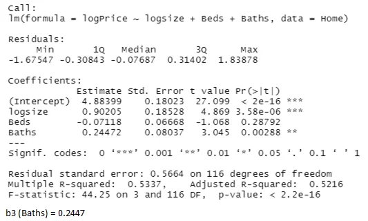
After transformation of Price and Size variables, the computed coefficients for the variables used while fitting a linear regression equation to predict price as the model 1 is as follows;

b0 (intercept) = 4.8840

b1 (size) = 0.9021

b2 (Beds) = -0.0712

Question 5

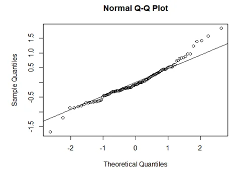
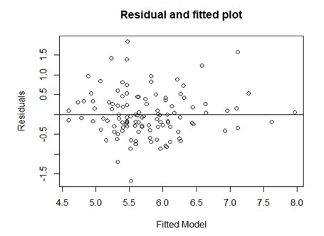
Residual diagnostic plots:

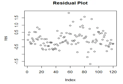
The Shapiro-Wilk test for normality for the residuals in this model are as shown in the figure below; The

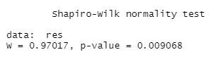
P value is 0.0091

Question 6

From the QQ-plot, residual plot, residual vs fitted plot, the top 3 observations that would impact the conclusions include;

From residual plots; 2

From residual and fitted plots; 7

From normal QQ-plot; 7

Question 7

When we run a second model without the outliers/extreme values, the computed regression coefficient values are as shown in the figure below;

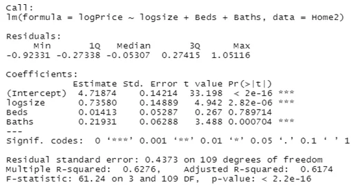
From the computed model above, removing the outliers makes the model better since we now have an r squared value of 0.6276 compared to our previous model 0.5337 showing that 62.8% of the variation in the price of houses in the model is explained by the variables. Removing outliers improves the model.

Question 8

From Model 1 = 0.2 * 0.9021 = 0.1804, which is 18.04%.

Question 9

The calculated effect above means that for an increase in 20% in home size, this would lead to an increase by 18.04% of the house price.

Question 10

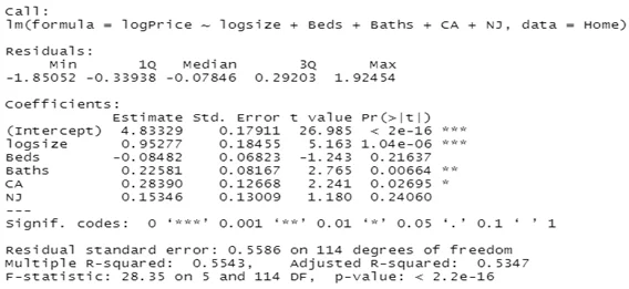
The difference between CA and NJ = 0.1304.

Question 11

The effect computed above shows than on average, the house price in California is 13.04% higher than the house price in New Jersey.

Question 12

The difference in multiple R squared = 0.5543 (in model 3) – 0.5337 (in model 2) = 0.0206.

Question 13

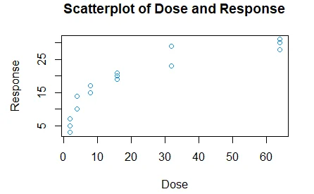
From the scatterplot and the coefficient estimate, there is a positive non-linear relationship between the covariate and response

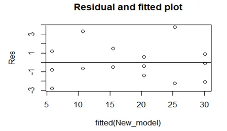
Question 14

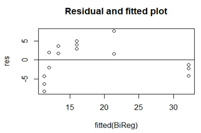
From the residual’s vs fitted values plot, there appears to be a problem.

Question 15

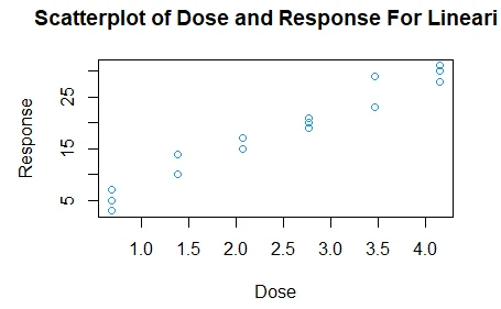
Yes, there is a linear relationship hence a linear model is appropriate.

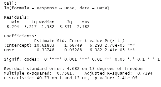
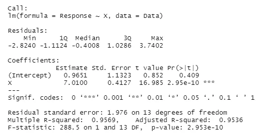
Question 16

b0 = 0.9651

b1 = 7.010

Multiple R squared = 0.9569

P-value of the b1 coefficient = 2.95e – 10

Question 17

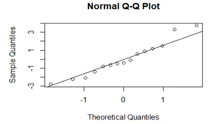
The Linear model does not seem appropriate since it has too many outliers. The normality assumption appears to be violated from the QQ-plot.

Question 18

For 5% change in log Dose = 0.05 * 7.010 = 0.3505 = 35.05% change in the response.

Question 19

The 95% confidence interval for the slope parameter in the model above is calculated as follows;

7.010+1.960* 0.417= (6.1927, 7.8273)

Question 20

Yes, we reject the null hypothesis since at 5% significance level, the computed P-value is lower than 0.05.

Question 21

X bar = 20

Y bar = 58

Sx = 6.758

Sy = 8.775

Syy = 462

Standard error of the intercept;

(t=b/SEb) = (6.075=35.1533/SEb) = 5.7866

t-value of x variable = 1.1423/0.2761 = 4.1373

the regression equation is as follows;

Y= 35.1533 + 1.1423X

The residuals sum of squares = (-0.99635)2+ (-1.71898)2+(5.9964)2+ (-0.5730)2+ (-6.8577)2+(0.00365)2+ (4.146)2= 104.450

SSR = SST- SSE = 462 – 104.450 = 357.55

SST = Syy = 462

Multiple R squares = 1-(SSE/SST) = 1 – (104.450/462) = 0.7749

Adjusted R squared = 0.7299

P-value of the F-test = 009018.