Assignment on Graphical Analysis of Hypothesis
Item #5 Graphs: Create a series of graphs (histograms, polygons, bar graphs, etc.) that summarize your findings in items 3 and 4. In other words, create graphs that compare the means and standard deviations of the dependent variable by the levels of the independent variable of interest. Discuss your findings. items 3 and 4 are below and info or background info for the problem is at the very bottom under items 3 and 4. The only thing I need help solving and creating is this item #5 parts regarding graphs and summarization. These numbers are based on 29 students who completed a survey in my class if that helps.
item #3 Measures of Central Tendency-
Research question: What determines one’s GPA?
Hypothesis: Those who are younger than 25, sit in the front of the class and have a study partner will be more likely to have a better grade than people who are opposite.
Independent variable:
1. Studying
2. Work environment
3. Age
How do the variables of (IV1) studying, (IV 2) Work environment, and (IV 3) Age effect (DV)Grade point Average ?
Age:
People that are above 25
People that are below 25
Work environment:
People that sit in the front
People that sit in the middle
People that sit in the back
Studying:
People that have a study partner
People that don’t have a study partner
SOLUTION
This section presents a graphical analysis of the hypothesis by comparing the mean, standard deviation, and distribution of the respondent's CGPA based on their age, work environment, and studying.
Effect of Age on CGPA
We used graphs to compare the CGPA of students above 25 years to those below 25 years. We hypothesized that students below 25 years will have high CGPA than respondents above 25 years. Figure 1 shows the histogram of the distribution of CGPA by age.
Fig 1: Histogram of CGPA by Age
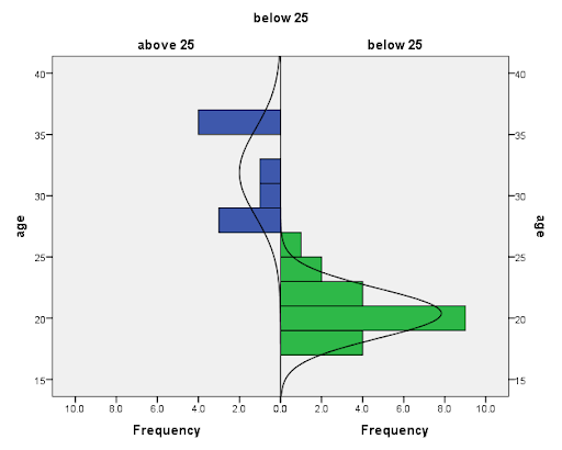
The figure shows that while the CGPA of students below 25 years is normally distributed and less spread out, the CGPA of students above 25 years is not normally distributed and is more spread out.
Fig 2: Box plot of distribution of CGPA by Age
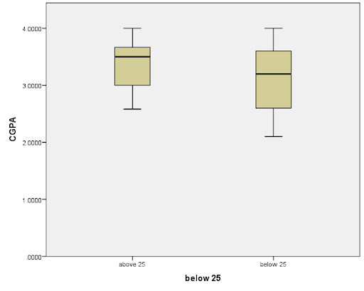
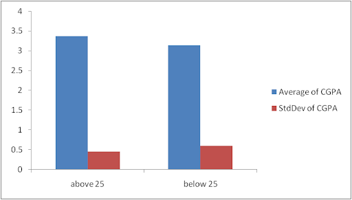
Fig 3 is a bar chart showing means and standard deviation of CGPA by age. The result shows that average CGPA is higher for respondents above 25 years than respondents below 25 years. Conversely, standard deviation is higher for respondents below 25 years than for respondents above 25 years. This means that there is high variation in CGPA within respondents who are less than 25 years than among respondents who are above 25 years.
Conclusion
The result shows that age affects CGPA but is contrary to our hypothesized relationship as we see that respondents above 25 years have high CGPA than respondents below 25 years but not the other way round.
CGPA and Work Environment
We hypothesized that respondents who sit in the front should have high CGPA than others whether they sit in the middle or at the back. Fig 1 shows the histogram of the distribution of CGPA across the three categories. The result shows that while the CGPA of respondents who sits in the front and middle does not seem to follow a normal distribution, the CGPA of respondents who sit at the back also does not follow a normal distribution. The CGPA of respondents who sits at the front is less spread out than others.
Fig 4: Histogram of CGPA by Work Environment
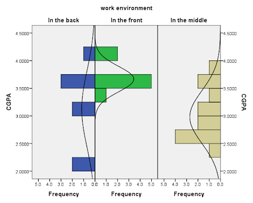
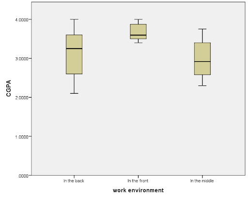
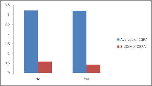
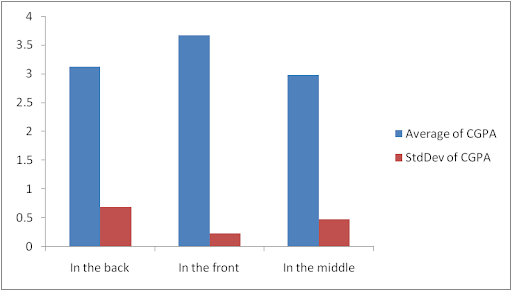
Fig 7 presents the bar chart of means and standard deviation of CGPA across work environment. The result shows that respondents who sit in the front have the highest average CGPA followed by those who sit at the back. On the other hand, the variation in CGPA is the lowest for those who sit at the front as they have the lowest standard deviation while the highest variation is found for respondents who sit at the back.
Fig 6: Bar Chart Showing Means and Standard deviations of CGPA by age
Conclusion
The result shows that work environment affects CGPA as people who sits in the front has the highest average and median CGPA. Thus, the hypothesis is confirmed.
Effect of Studying on CGPA
We hypothesized those respondents who have study partner have high CGPA than those without study partner. Figure 7 shows the histogram of the distribution of CGPA by studying.
Fig 7: Histogram of CGPA by Studying
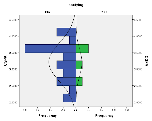
The figure shows that while the CGPA of those who have study partners is normally distributed and less spread out, the CGPA of those without study partners is not normally distributed and is more spread out.
Fig 8: Box plot of the distribution of CGPA by Studying
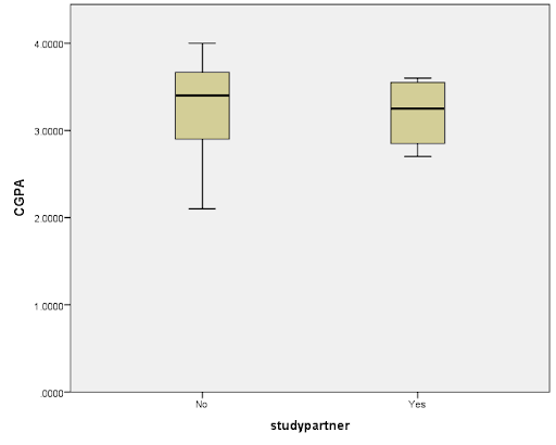
Figure 8 presents the box plot showing the distribution of CGPA by study. The distribution of respondents who have study partners is confirmed to be normal as we see that the median and quartiles are almost evenly spaced. We also discovered from the plot that the median CGPA for respondents who have study partners is not much different from those who have a study partners.
Fig 9: Bar Chart Showing Means and Standard deviations of CGPA by study