Exploratory analysis homework solution

Exploratory analysis using R Studio on taxi demand and pricing

Here we will use a dataset from the TLC website to analyze the demand and pricing of taxis. We will determine how much one is supposed to pay at a time. 

Report on Exploratory Analysis using R Studio

Abstract

Transportation is important in the modern city and taxi is the major means of transportation in large cities. It is important to know factors that drive demand for appropriate planning. The objective of this study is to explore factors that influence the amount spent by passengers on a taxi trip. To achieve this, we used data from New York City for December 2020. The data contains over a million records collected on trips that occurred within that period. Exploratory analysis and summary statistics were used to explore relationships after some preprocessing of data like data cleaning, subsetting, and variable selection have been conducted. The result found that payment type, distance covered, day of the week, and hour of the day are important variables that determine the amount spent on taxi trips. We also found that spending is lower around the early morning until the second hour afternoon. Thus, the trip charges being lowered at this period may motivate some passengers to reschedule their trip and this reduces the burden during the rush hour. The work is of benefit to TLC and companies that provide car hire service in allocating their cars in the most efficient, profit-maximizing manner.

Introduction

Transportation plays a major role in large modern cities. It is important for the conveyance of people and goods from their source to the destination. The modes of transportation are diverse. However, taxi plays a major role in commuting people in large cities around the world. It provides convenience, accessibility, and privacy to the passengers (Natasha and Velu, 2020). The decision to experience the taxi service by private car users hinges closely on the competitiveness and reasonableness of taxi pricing.

The New York Taxi and Limousine Commission provides data on the volume of taxi trips service that was offered. The data provides an opportunity to gain insights into the factors that determine the cost of trips and the distance traveled. Moreover, the peak period and the period when taxi hire is low and so on. Data of such nature makes planning easy on the dissemination of taxis around the city and over the twenty-four hours window. Thus, analyzing the demand for transportation is an important first step in ensuring taxi service is top-notch.

Many factors may influence the trip fare chief of which is the trip distance but other factors include the convenience enhancing services offered on the trip, number of passengers, and so on. Based on the preceding argument, this report seeks to analyze the New York city TLC data for December 2020 to determine the important factors that influence the amount charged for fares. The objective of the study is to conduct an exploratory analysis to determine factors that affect fare charges for NYC taxis.

Data

The dataset was retrieved from the TLC website at “https://www1.nyc.gov/site/tlc/about/tlc-trip-record-data.page “. The dataset consists of records on trip carried out by yellow taxis and include information such as time of pick-up and drop, distance, fare amount as well as other amount and total amount. The data were collected by technology providers who are authorized under the “Taxicab & Livery Passenger Enhancement Programs (TPEP). The yellow taxi data used for this work is provided by two technology providers which are: Creative Mobile Technologies and Verifone incorporated. This is done through installed taximeters that automatically collect trip data between when the meter is engaged and disengaged. Only the number of passengers is collected by the driver.

The dataset for December 2020 contains 1,461,897 observations and 17 variables which are explained in the table below

*source:https://www1.nyc.gov/assets/tlc/downloads/pdf/data_dictionary_trip_records_yellow.pdf

There is one variable that is in the dataset (congestion surcharge) which documentation is not provided by the above source. Thus, we remove the variable from the dataset.

Methods

Data Cleaning

The data was collected in a structured form in .csv format. However, the summary statistics of the variables revealed some deficiencies in the data. For example, the distance covered, the minimum is zero which means the meter must have been activated in error or faulty or the trip was abolished. Using the length function combined with which function in R, we found that 17,353 observations were found to have zero distance. Such observations were removed as part of the data cleaning process. Moreover, fare amount, total amount, and other charges have their minimum as a negative value which is not possible for variables of such nature. Using a similar function, we found 8,375 observations with negative fare amount and 503observations with the negative total amount. Those observations were removed as well as other negative or zero charges on other categories of fees (e.g. toll charges). The removal was done using the filter function from the dplyr package in R

Moreover, we found that there are outliers in some of the continuous variables like fare_amount, trip_distance, and total_amount. The presence of outliers will distort relationships and summary statistics like the mean. Thus, removal of those outliers’ values is necessary. The outliers were detected using boxplot, then we used the IQR rule in conjunction with the filter function from dplyr package to remove the outliers. In the same vein, some variables have missing values. The observations where one entry is missing were also omitted from the analysis. This removal was done using na. omit function. We opted against imputation because one of the variables is categorical and imputing it may bias results like when we group according to the category while the other is just a code variable that is not necessary for analysis. At the end of the data cleaning exercise, we were left with1,273,612 observations.

Type Conversion

In this section, we converted some variables that were not given in the appropriate type to the appropriate type. The first variable we converted is the pickup and dropoff date and time-variable entered as a character to DateTime variable in R. This is necessary for R to recognize it as a date variable and we can easily calculate the hour of the day or the day of the week from it. We used the as.POSICTcx function to achieve this. Moreover, the ratecodeidand payment type was converted from numeric variables to factor variables to reflect the appropriate level of measurement. The factor function was used to achieve conversion from numeric to factor variables.

Data subset selection and/or subsampling

The variable measuring the payment type has six categories. However, four of the categories (no charge, dispute, voided trips, and unknown) are not necessary for the study. Thus, we use the filter function to subset the data to include only passengers who paid by cash or credit card. We were left with 1,266,449 observations.

Variable selection and/or transformation

Variable selection helps to determine which variables are important for the total amount paid by passengers from the candidate independent variables that we have. The independent variables we have are passenger count, distance, the type of rate, the payment type, hour of the day, day of the week, weekend/weekdays, and day/night and vendor ID. Not all these variables will be important for the amount of fare. For example, we do not expect the vendor to have an effect on the amount paid by trip as they only provide technology to record data. Thus, we used a stepwise regression model for variable selection. This method involves starting from a null model and adding each of the independent variables one after the other. The process stops when the remaining variables are not significant based on defined criteria. We use the step function along with the lm function to achieve this objective. The hour and day of the week variable were calculated using the hour and day function from the lubridate package. The ifelse function was used to categorize to weekend/weekday and to day/night

Group-based data summarization

The total amount paid on a trip usually varies due to some characteristics. Charges may be lower at some time of the day because they are off-period while higher at the rush hours. Similarly, the fare may be different on weekdays than weekends or based on the number of passengers. Group-based summarization is used to capture such variation between groups. Summary statistics were calculated for the total amount paid by passengers based on the categorical variables that were deemed important from the selection step. The group_by and summarize function from dplyr were combined to create the group-based summary.

Exploratory visualization using ggplot2

After we have determined that the important variables that determine the total amount paid for the trip are distance, rate type, payment type, day of the week, an hour of the day, and vendor type, we proceed to visualize the relationship with ggplot2. The appropriate visualization depends on the variable types. The distance variable is continuous, so a scatterplot is suitable to explore its relationship with the total amount paid. A box plot is used to visualize the relationship between total amount and vendor type. A pie chart is used for payment type and rate type while a bar chart is used for the day of the week and hour. In addition to the ggplot, geom._point was used to plot the scatterplot while geom._smooth plot the trend line. geom._bar was used for the bar char while coord_polar was added to geom_bar to give a pie chart.

Result and Discussion

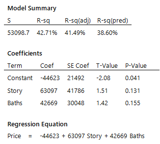
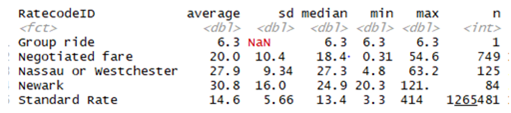
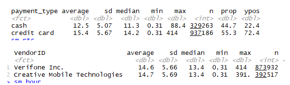
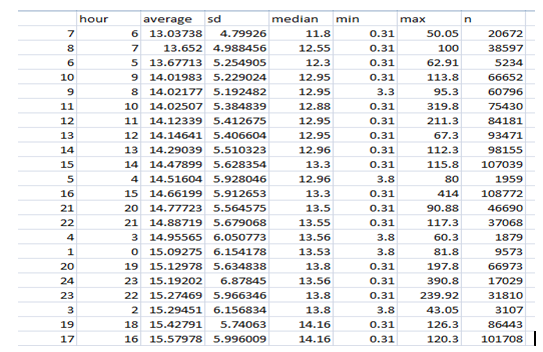
The group-based summary statistics show that the average total amount spent based on weekdays ranges from $14.3(sd=5.58/5.71) for Saturdays and Sundays respectively to $15 (sd=5.83) for Fridays. This means there is more spending during weekdays than weekends. The bar grain fig 1 however shows not much variation in spending through weekdays as the difference between the smallest and highest is not up to a dollar. Average spending ranges from $13.04 on the seventh hour of the day (i.e. 7 A.M) to $15.71 (sd=5.99) for the 17th hour of the day (5 PM). The pattern discovered here is that spending is low from dawn till around 2 PM as average spending between this periods took the bottom 10 rankings of the average spending while at the top is mixed between evening period and night period. Credit card users (M=15.4, SD=5.07) spent higher than passengers who paid in cash (M=12.5, SD=5.67). The pie chart shows that credit card users spent 55.29% of average total spending while those that spent in cash spent 44.71%. credit card users may spend higher because of their ability to pay even when they don’t have enough money in their account. This raises their probability to hire more. Even though the standard rate is the most prevalent, it ranked fourth of five contributing only 13.5% of average total spending. The Newark rate has the highest average total spending of $30.8 constituting 27.58% of overall average total spending. The scatter plot in fig 1 shows that the relationship between average total spending and trip distance. There is a positive relationship even though the slope of the fit line does not suggest a strong relationship but a careful look shows a tendency of an upward sloping curve. Finally, the average fare amount does not seem to vary much with vendor ID which is not unexpected.

Conclusion

This project sets out to explore variables that determine the amount spent on a trip on New York City yellow taxi in order to provide insights for the TLC and other private hire companies which features to focus on. Using data for December 2020 an exploratory analysis, we found through the variable selection that the amount paid varied by distance, payment type, rate type, day of the week, and hours of the day. However, the exploratory analysis shows variation among categories within each of the variables is slight. Thus, the result is not final as further analysis is needed to explore other features that may be important.

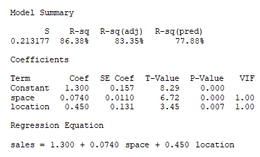
Fig 1: 

nyctrip<-read.csv("yellow_tripdata_2020-12.csv") head(nyctrip,2) dim(nyctrip) summary(nyctrip) nyctrip=nyctrip[,-18] dim(nyctrip) length(which(nyctrip$trip_distance==0)) length(which(nyctrip$fare_amount<=0)) length(which(nyctrip$total_amount==0)) library(dplyr) nyctrip_clean=nyctrip%>%filter(trip_distance>0)%>% filter(fare_amount>0)%>% filter(total_amount>0)%>% filter(extra>=0)%>% filter(mta_tax>=0)%>% filter(improvement_surcharge>=0)%>% filter(tolls_amount>=0)%>% filter(tip_amount>=0) summary(nyctrip_clean) boxplot(nyctrip_clean$fare_amount) boxplot(nyctrip_clean$trip_distance) boxplot(nyctrip_clean$total_amount) library(EnvStats) int=iqr(nyctrip_clean$fare_amount) tile<-quantile(nyctrip_clean$fare_amount,probs=c(.25,.75),na.rm=F) up=tile[2]+3*int low=tile[2]-3*int nyctrip_clean=nyctrip_clean%>% filter(fare_amount>low&fare_amount% filter(trip_distance>low&trip_distance%filter(payment_type=="credit card"| payment_type=="cash") dim(nyctrip_clean2) #Group-based data summarisation library(dplyr) library(lubridate) nyctrip_clean2$day <- factor(day(nyctrip_clean2$tpep_pickup_datetime)) nyctrip_clean2$dayofweek <- factor(wday(nyctrip_clean2$tpep_pickup_datetime, label = TRUE)) nyctrip_clean2$hour<-factor(hour(nyctrip_clean2$tpep_pickup_datetime)) nyctrip_clean2$weekend<-factor(ifelse(nyctrip_clean2$dayofweek=="Sat"| nyctrip_clean2$dayofweek=="Sun","weekday","weekend")) nyctrip_clean2$hours=as.numeric(nyctrip_clean2$hour) nyctrip_clean2$time<-factor(ifelse(nyctrip_clean2$hours>6& nyctrip_clean2$hours<19,"day","night")) nyctrip_clean2$VendorID=factor(nyctrip_clean2$VendorID,levels=c(1,2), labels=c("Creative Mobile Technologies","Verifone Inc.")) regdt=nyctrip_clean2[,c(1,4:7,10,17,19:21,23)] set.seed(456) regdt=sample_n(regdt,10000,replace = T) mod=lm(total_amount~.,data=regdt) summary(step(mod)) sm_dow<-nyctrip_clean2%>%group_by(dayofweek)%>% summarize(average=mean(total_amount),sd=sd(total_amount),median=quantile(total_amount,prob=0.5),min=min(total_amount),max=max(total_amount),n=length(total_amount)) sm_hour<-nyctrip_clean2%>%group_by(hour)%>% summarize(average=mean(total_amount),sd=sd(total_amount),median=quantile(total_amount,prob=0.5),min=min(total_amount),max=max(total_amount),n=length(total_amount)) sm_vendor<-nyctrip_clean2%>%group_by(VendorID)%>% summarize(average=mean(total_amount),sd=sd(total_amount),median=quantile(total_amount,prob=0.5),min=min(total_amount),max=max(total_amount),n=length(total_amount)) sm_rtc<-nyctrip_clean2%>%group_by(RatecodeID)%>% summarize(average=mean(total_amount),sd=sd(total_amount),median=quantile(total_amount,prob=0.5),min=min(total_amount),max=max(total_amount),n=length(total_amount)) sm_ptype<-nyctrip_clean2%>%group_by(payment_type)%>% summarize(average=mean(total_amount),sd=sd(total_amount),median=quantile(total_amount,prob=0.5),min=min(total_amount),max=max(total_amount),n=length(total_amount)) ##ggplot #scatterplot library(ggplot2) p1<-ggplot(nyctrip_clean2, aes(x =trip_distance, y = total_amount)) + geom_point(color = "grey60") + geom_smooth(se = FALSE, method = "lm", formula = y ~ x, color = "#0072B2")+ scale_x_continuous(name = "Distance covered\n(miles)") + scale_y_continuous(name = "Total amount paid for trip\n($)") + theme_minimal() + theme(text = element_text(size=13), legend.position = "none") sm_ptype<- sm_ptype %>% arrange(desc(payment_type)) %>% mutate(prop = average/ sum(sm_ptype$average) *100) %>% mutate(ypos = cumsum(prop)- 0.5*prop ) p2<-ggplot(sm_ptype, aes(x="", y=average, fill=payment_type)) + geom_bar(stat="identity", width=1, color="white") + coord_polar("y", start=0) + theme_void() + geom_text(aes(label =paste0(round(prop,2),"%")),position=position_stack(vjust=0.5))+ scale_fill_brewer(palette="Set1") sm_rtc<- sm_rtc%>% arrange(desc(RatecodeID)) %>% mutate(prop = average/ sum(sm_rtc$average) *100) %>% mutate(ypos = cumsum(prop)- 0.5*prop ) p3<-ggplot(sm_rtc, aes(x="", y=average, fill=RatecodeID)) + geom_bar(stat="identity", width=1, color="white") + coord_polar("y", start=0) + theme_void() + geom_text(aes(label =paste0(round(prop,2),"%")),position=position_stack(vjust=0.5))+ scale_fill_brewer(palette="Set1") p4<-ggplot(data=sm_dow,aes(x=dayofweek,y=average))+ geom_bar(stat="identity")+ labs(x="day of the week",y="Average Total amount paid for trip")+ theme_minimal() p5<-ggplot(data=sm_hour,aes(x=hour,y=average))+ geom_bar(stat="identity")+ labs(x="day of the week",y="Average Total amount paid for trip")+ theme_minimal() sm_vendor<- sm_vendor%>% arrange(desc(VendorID)) %>% mutate(prop = average/ sum(sm_vendor$average) *100) %>% mutate(ypos = cumsum(prop)- 0.5*prop ) p6<-ggplot(sm_vendor, aes(x="", y=average, fill=VendorID)) + geom_bar(stat="identity", width=1, color="white") + coord_polar("y", start=0) + theme_void() + geom_text(aes(label =paste0(round(prop,2),"%")),position=position_stack(vjust=0.5))+ scale_fill_brewer(palette="Set1") library(gridExtra) grid.arrange(p1,p2,p3,p4,p5,p6)