-
Home
-
Empirical Methods Assignment Solution In Finance
Empirical Methods in Finance Using R Programming
Please use R to solve these problems. You can just hand in one set of solutions that has all the names of the contributing students in each group. Use the electronic drop box to submit your answers. Submit the R file and the file with a short write-up of your answers separately.
[The quality of the write-up matters for your grade. Please imagine that you‘re writing a report for your boss at Goldman when drafting answers to these questions. Try to be clear and precise.]
Building a Simple auto Correlation-based Forecasting Model
Fama and French(20fi†)propose a five-factor modelforexpectedstockreturns.One of the factors is based on cross-sectional sorts of firm profitability. In particular, the factor portfolio is long firms with high profitability (high earnings divided by book equity¡ high ROE) and short firms with low profitability (low earnings divided by book equity¡ low ROE). This factor is called RMW – Robust MinusWeak.
1. Go to KenFrench‘s Data Library(googleit)anddownloadtheFama/French†Factors (2x3)inCSVformat.Denote the time series of value-weighted monthly factor returns for the RMW factor from fi963.0F-2020.fi0as"rmw."Plot the time series, give the annualized mean and standard deviation of this return series
2. Plotthefistto60thorderautocorrelationsofrmw.Also plot the cumulative sum of these autocorrelations(that is, the observation is the sum of the first †auto correlations, the fifth observation is the sum of the first auto correlations, etc.). Describe these plots. In particular, do the plot at the predictability of the factor returns? What are the salient patterns, if any?
3. Perform a Ljung-Box test that the first 6 autocorrelations jointly are zero. Write out the form of the test and report the p-value. What do you conclude from this test?
4. Based on your observations in (2) and (3), propose a parsimonious forecasting model for rmw. That is, for the prediction model
vmut‡fi=ØJıt‡ot‡fi, (fi)
where the first variable in ıtis a fi for the intercept in the regression. Choose the remaining variables in ıt–it could be only one more or a longer K×five factor. While this analysis is an in-sample, I do want you to argue for your variables by attaching a "story" to your model that makes it more exact and believable. (PS: This question is purposefully a little vague. There is not a single correct answer here, just grades of more to less reasonable as in the real world).
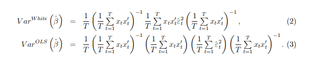
5. Estimate the proposed model.Report Robust(White)standard errors for ؈, as well as the regular OLS standard errors. In particular, from the lecture notes, we have that
(In asymptotic standard errors, we do not adjust for degrees of freedom which is why we simply divide by T
Non-stationarity and Regression Models
1. Simulate f time series observations of each of the following two return series N times:
vfi,t = µ ‡aofi,t,
vX,t = µ‡aoX,t, (4)
whereµ=0.5%,a=Œ%,and the residuals are uncorrelated standard Normals. Let
f = 600 and N = fi0, 000. For each of the N time series, regress:
vfi,t=α‡ØvX,t‡ot, (†)
and save the slope coefficient as Ø(n),wheren=fi,...,N.Give the mean and standard deviation of Ø across samples n and plot the histogram of the fi 0,000Ø‘s.Does this correspond to the null hypothesis Ø=0?Do the regress standard errors look ok?
2. Next, construct N price sample of length f based on each return using:
pfi,t = pfi,t—fi ‡ vfi,t,
pX,t = pX,t—fi ‡ vX,t, (6)
using pfi,O=pX,O=0as the initial condition.Now,repeat the regression exercise using the regression:
pfi,t=α‡ØpX,t‡ot. (F)
Again report the mean and standard deviation of the N estimated Ø‘s and plot the histogram. Does this correspond to the null hypothesis Ø = 0? Do the regression standard errors look ok? Explain what is going on here that is different from the previous return-based regressions.
set.seed(1)
##############################Q2 part 1
mu<-0.5
sigma<-4
t<-600
N<-10000
beta<-numeric(N)
r1t<-numeric(t)
r2t<-numeric(t)
for ( i in 1:N)
{
  r1t<-mu+sigma*rnorm(t,0,1)
  r2t<-mu+sigma*rnorm(t,0,1)
  mod<-lm(r2t~r1t)
  beta[i]<-mod$coefficients[2]
}
mean(beta)
sd(beta)
hist(beta)
t.test(beta, mu = 0, alternative = "two.sided")
##############################Q2 part 2
p1_vec<-function(t)
{
  r1t<-mu+sigma*rnorm(600,0,1)
  y1<-numeric(t+1)
  y1[1]<-0
  for(i in 2:t+1)
  {
    #since for y1 i=1 is same as p1,0 but in case of r1t i=1 is same as t=1 since y1 array starts from
    # 1 and goes upto t+1 but r1t goes from i=1 to i=t
    y1[i]<-y1[i-1]+r1t[i-1]
  }
  return(y1)
}
p2_vec<-function(t)
{
  r2t<-mu+sigma*rnorm(t,0,1)
  y2<-numeric(t+1)
  y2[1]<-0
  for(i in 2:t+1)
  {
    #since for y2 i=1 is same as p1,0 but in case of r2t i=1 is same as t=1 since y2 array starts from
    # 1 and goes upto t+1 but r2t goes from i=1 to i=t
    y2[i]<-y2[i-1]+r2t[i-1]
  }
  return(y2)
}
betas<-numeric(N)
for ( i in 1:N)
{
  p1<-p1_vec(t)
  p2<-p2_vec(t)
  mod<-lm(p1~p2)
  betas[i]<-mod$coefficients[2]
}
mean(betas)
sd(betas)
hist(betas)
plot(mod)
t.test(betas, mu = 0, alternative = "two.sided")
set.seed(1)
########################Q1
df<-read.csv("F-F_Research_Data_5_Factors_2x3.csv",skip=2)
df<-df[1:688,]
library(anytime)
df$X<-anydate(df$X)
names(df)[names(df)=="X"]<-"Date"
tse<-ts(df$RMW,start=c(1963, 7), end=c(2020, 10), frequency=12)
plot.ts(tse)
row.names(df) <- levels(df$Date)[df$Date]
library(PerformanceAnalytics)
Return.annualized(df$RMW,scale=12)
sum(is.na(df$RMW))
df$RMW<-as.numeric(df$RMW)
a<-acf(df$RMW,lag.max = 60)
plot(a)
cum_acf<-a$acf[2:61]
cum_acf_calculated<-cumsum(cum_acf)
cum_acf
x<-1:60
plot(x,cum_acf_calculated,xlab = "lag",ylab = "Cummulative ACF")
Box.test(df$RMW,lag=6)
##############################Q2 part 1
mu<-0.5
sigma<-4
t<-600
N<-10000
beta<-numeric(N)
r1t<-numeric(t)
r2t<-numeric(t)
for ( i in 1:N)
{
  r1t<-mu+sigma*rnorm(t,0,1)
  r2t<-mu+sigma*rnorm(t,0,1)
  mod<-lm(r2t~r1t)
  beta[i]<-mod$coefficients[2]
}
mean(beta)
sd(beta)
hist(beta)
t.test(beta, mu = 0, alternative = "two.sided")
##############################Q2 part 2
p1_vec<-function(t)
{
  r1t<-mu+sigma*rnorm(600,0,1)
  y1<-numeric(t+1)
  y1[1]<-0
  for(i in 2:t+1)
  {
    #since for y1 i=1 is same as p1,0 but in case of r1t i=1 is same as t=1 since y1 array starts from
    # 1 and goes upto t+1 but r1t goes from i=1 to i=t
    y1[i]<-y1[i-1]+r1t[i-1]
  }
  return(y1)
}
p2_vec<-function(t)
{
  r2t<-mu+sigma*rnorm(t,0,1)
  y2<-numeric(t+1)
  y2[1]<-0
  for(i in 2:t+1)
  {
    #since for y2 i=1 is same as p1,0 but in case of r2t i=1 is same as t=1 since y2 array starts from
    # 1 and goes upto t+1 but r2t goes from i=1 to i=t
    y2[i]<-y2[i-1]+r2t[i-1]
  }
  return(y2)
}
betas<-numeric(N)
for ( i in 1:N)
{
  p1<-p1_vec(t)
  p2<-p2_vec(t)
  mod<-lm(p1~p2)
  betas[i]<-mod$coefficients[2]
}
mean(betas)
sd(betas)
hist(betas)
plot(mod)
t.test(betas, mu = 0, alternative = "two.sided")