Instructions
1. The primary objective of the Study on the Efficacy of Nosocomial Infection Control (SENIC Project) was to determine whether infection surveillance and control programs have reduced the rates of nosocomial (hospital-acquired) infection in United States hospitals. This data set consists of a random sample of 113 hospitals selected from the original 338 hospitals surveyed. Each line of the data set has an identification number and provides information on 11 other variables for a single hospital. The data presented here are for the 1975-76 study period. Please download hospital.xlsx from Blackboard. The dataset contains 12 variables shown below.
| 1 Identification number: 1-113
2 Infection risk: Average estimated probability of acquiring infection in hospital (in percent) 3 Length of stay: Average length of stay of all patients in hospital (in days) 4 Age: Average age of patients (in years) 5 Routine culturing ratio: Ratio of number of cultures performed to number of patients without signs or symptoms of hospital-acquired infection, times 100 6 Routine chest X-ray ratio: Ratio of number of X-rays performed to number of patients without signs or symptoms of pneumonia, times 100 7 Number of beds: Average number of beds in hospital during study period 8 Medical school affiliation: 1=Yes, 2=No 9 Region: Geographic region, where: 1=Northeast, 2=Northcentral, 3=South, 4=West 10 Average daily census: Average number of patients in hospital per day during study period 11 Number of nurses: Average number of full-time equivalent registered and licensed practical nurses during study period (number full time plus one half the number part time) 12 Available facilities and services: Percent of 35 potential facilities and services that are provided by the hospital |
1.1 Import the dataset into SPSS. Make sure you correctly specify the Measure for each variable. Please add Values for two categorical variables – medical school affiliation and region. Report descriptive measures and create graphical displays for the following variables – length, age, infection risk, available facilities and services, and number of beds. Provide a summary of your findings (no more than 200 words) based on the descriptive statistics and displays.
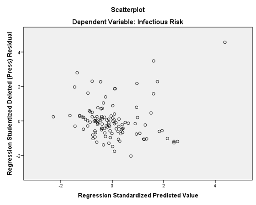
1.2 Confirmatory approach: Consider a regression model with infectious risk against age, routine culturing ratio, average daily census, available facilities and service, and Medical school affiliation. Provide a write-up of your findings (no more than 300 words) in APA format to address the following three issues.
• Assumption of homoscedasticity, assumption of normality, independence of error terms (i.e. autocorrelation), and collinearity between predictors.
• Provide the prediction equation. Interpret the value of unstandardized coefficients within the context.
• Identify any outlier or influential point based on Cook’s D and standardized DfBeta.
1.3 exploratory approach: Use either forward or stepwise selection method to find the best set of predictors for explaining length of stay. Consider all other variables as candidate predictors excluding medical school affiliation and region. Describe the variable selection procedure and report the final model (no more than 200 words). Hint: Make sure you adjust the tolerance level to be 0.10.
1.4 Consider a regression model with infectious risk against average daily census and Medical school affiliation. Assume there is no interaction between Medical school affiliation and daily census (i.e., equal slopes). Provide separate prediction equations for those affiliated with a medical school (yes) and those are not affiliated (no). Report your findings.
2. A researcher would like to investigate factors that are related to the years of graduate school for a student and number of students graduating. The data responses are stored in Graduate.sav. Four variables are measured.
| year: years of graduate school (values range from 1 year to 14 years)
university: 1 – UC, Berkeley; 2 – Columbia University; 3 – Princeton University residence: 1 – permanent residents; 2 – temporary residents events: number of students graduating in each category For example, the first line of data would read: there are 31 students, who are permanent residents and spent one year in graduate school, are graduating in UC, Berkeley. |
2.1 Are years of graduate school differ among students in different universities and with different residence status? Use appropriate GLM method to examine the main effect of university, main effect of residence status, and their interaction effect on years of graduate school. Create an APA style summary (no more than 200 words) and include the test result on homogeneity assumption, ANOVA summary table, interpretation of overall model usefulness as well as main and interaction effects based on F test and effect size measures.
2.2 This researcher is also interested in the relationship between number of students graduating and their years of graduate school. Create an appropriate graphical display to show this relationship, and summarize your observations (no more than 100 words). Then use an appropriate statistical measure to report the linear association between these two variables, and interpret the value within the context (no more than 100 words).
2.3At last, this researcher wants to examine whether number of students graduating differs by university and residence status. Use appropriate GLM method to examine the main effect of university, main effect of residence status, and their interaction effect on number of students graduating. If the interaction effect is significant, conduct simple effect analysis. Provide a summary to describe your analysis and all of the findings (no more than 300 words).
3. A group of researchers is asked to examine the effect of a new brand of Margarine (called as Clora Margarine) on the cholesterol measures. Eighteen participants were recruited through a random sampling process, and used Clora Margarine for 8 weeks. Their cholesterol was measured before the special diet, after 4 weeks, and after 8 weeks. The data responses are stored in Cholesterol.sav.
3.1 Report descriptive measures and create graphical displays
(a) Create a table to display descriptive measures for cholesterol levels at three different time points (i.e., before, after 4 weeks, and after 8 weeks).
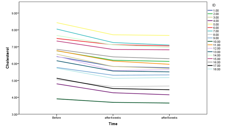
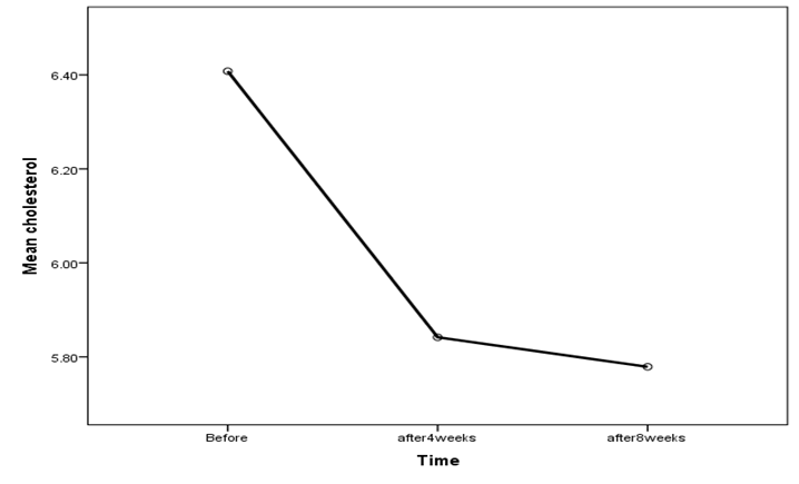
(b) Two graphs are shown below. The first graph displays changes in cholesterol measures across three-time points for each participant. The second graph only indicates the average cholesterol measure at each time point. Note that the scale of the y-axis is different in these two plots. Please comment on the mean difference of cholesterol across three-time points as well as individual differences in the changes of cholesterol measures.
3.2Use appropriate GLM method to test whether change in mean cholesterol is significant across three time points. Provide an APA format write-up to summarize all the procedures in your analysis and general findings. Please at least cover the following information in your report.
- Assumption of sphericity.
- The F test and effect size measures for the main analysis. (Please make sure you use the most appropriate F statistic and corresponding degrees of freedom.)
- Conduct post hoc comparisons if applicable on cholesterol measures between each pair of time points using Sidak method. (Hint: Time is a within-subject factor. In SPSS, the Post Hoc option conducts post hoc comparisons for between-subject factors only.)
Assignment solution
Question 1.1
Table 1: Descriptive Statistics
| N | Minimum | Maximum | Mean | Std. Deviation | |
| Infectious Risk | 113 | 1.3 | 17.9 | 5.102 | 2.4735 |
| Length | 113 | 1.60 | 42.00 | 10.1073 | 4.18667 |
| Age | 113 | 38.8 | 65.9 | 53.232 | 4.4616 |
| Available facilities and services | 113 | 6 | 835 | ||
| Number of beds | 113 | 29 | 835 | 43.16 | 15.201 |
| Valid N (listwise) | 113 | 252.17 | 192.843 |
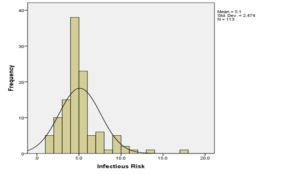
Fig 1: Histogram for infectious risk
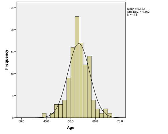
Fig 2: Histogram for Age
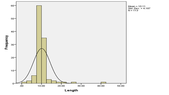
Fig 3: Histogram for Length
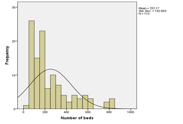
Fig 4: Histogram for Number of beds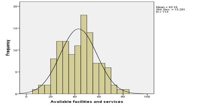
Fig 5: Histogram of available facilities and services
Table 1 above shows the descriptive statistics of the interest variables including the mean, standard deviation, and minimum and maximum values. The mean age of respondents is 53.23 while its standard deviation is 4.462. The average length of stay in the hospital is 10.11 while its standard deviation is 4.187. Infectious risk has a mean value of 5.10 and a standard deviation value of 2.474. The average number of beds in the hospital is 252.17 and its standard deviation is 192.843. Lastly, the available facilities and services have a mean of 43.16 and a standard deviation value of 15.201. To visualize all these variables the histogram bar chart was used with a super imposed normal curve which tells which the direction of their distribution. Only Age and available facilities and services were normally skewed to the left while other variables were skewed to the right.
Question 1.2
ANOVAa
| Model | Sum of Squares | df | Mean Square | F | Sig. |
| Regression | 104.885 | 5 | 20.977 | 3.867 | .003b |
| 1 Residual | 104.885 | 107 | 20.977 | ||
| Total | 685.251 | 112 |
| Model | R | R Square | Adjusted R Square | Std. Error of the Estimate |
| 1 | .391a | .153 | .113 | 2.3289 |
Coefficients'a
| Model | Unstandardized Coefficients | Standardized Coefficients | t | Sig | Correlations | Collinearity Statistics | ||||||
|---|---|---|---|---|---|---|---|---|---|---|---|---|
| B | Std. Error | Beta | Zero-order | Partial | Part | Tolerance | VIF | |||||
| 1 | (Constant) | .267 | 3.231 | .082 | .934 | |||||||
| Age | .114 | .051 | .206 | 2.231 | .028 | .179 | .211 | .198 | .925 | 1.081 | ||
| Routine culturing ratio | -.002 | .023 | -.007 | -.077 | .939 | -.031 | -.007 | -.007 | .874 | 1.144 | ||
| Average daily census | 006 | .002 | .402 | 2.587 | .011 | .313 | .243 | .230 | .329 | 3.044 | ||
| Available facilities and services | -.028 | .024 | -.175 | 1.207 | .230 | .178 | -.116 | -.107 | .376 | 2.657 | ||
| Medical school affiliation | -.669 | .796 | -.097 | -841 | .402 | -.221 | -.081 | -.075 | .593 | 1.686 | ||
| Residuals Statistics | |||||
|---|---|---|---|---|---|
| Minimum | Maximum | Mean | Std. Deviation | N | |
| Predicted Value | 2.886 | 9.336 | 5.102 | 9677 | 113 |
| Std. Predicted Value | -2,290 | 4.375 | .000 | 1.000 | 113 |
| Standard Error of Predicted Value | 266 | 1.102 | 505 | .182 | 113 |
| Adjusted Predicted Value | 2.809 | 7.816 | 5.078 | .9494 | 113 |
| Residual | -4.5034 | 8.6040 | 0000 | 2.2764 | 113 |
| Std. Residual | -1.934 | 3.694 | .000 | .977 | 113 |
| Stud. Residual | -2.014 | 4.194 | .005 | 1.026 | 113 |
| Deleted Residual | -4.8855 | 11.0873 | .0241 | 2.5141 | 113 |
| Stud. Deleted Residual | -2.044 | 4.566 | .012 | 1.052 | 113 |
| Mahal. Distance | .473 | 24.094 | 4.956 | 4.646 | 113 |
| Cook's Distance | .000 | .846 | .019 | .083 | 113 |
| Centered Leverage Value | .004 | .215 | .044 | .041 | 113 |
| Collinearity Diagnostics | |||||||||
|---|---|---|---|---|---|---|---|---|---|
| Model | Dimension | Eigenvalue | Condition Index | Variance Proportions | |||||
| (Constant) | Age | Routine culturing ratio | Average daily census | Available facilities and services | Medical school affiliation | ||||
| 1 | 1 | 5.273 | 1.000 | .00 | .00 | .01 | .00 | .00 | .00 |
| 2 | .390 | 3.679 | .00 | .00 | .02 | .22 | .01 | .01 | |
| 3 | .289 | 4.274 | .00 | .00 | .83 | .00 | ,00 | .01 | |
| 4 | .033 | 12.633 | .00 | .00 | .05 | .69 | .92 | .04 | |
| 5 | .013 | 20.256 | .04 | .16 | .00 | .07 | .06 | .87 | |
| 6 | .003 | 42.457 | .95 | .83 | .09 | .01 | .01 | .08 | |
| a. Dependent Variable: Infectious Risk | |||||||||
| Model Summary | ||||
|---|---|---|---|---|
| Mod el | R | R Square | Adjusted R Square | Std. Error of the Estimate |
| 1 | .473a | .224 | .217 | 2.1885 |
| 2 | .517b | .267 | .254 | 2.1366 |
| 3 | .546c | .298 | .278 | 2.1014 |
| 4 | .572d | .327 | .302 | 2.0665 |
b. Predictors: (Constant), Length, Average daily census
c. Predictors: (Constant), Length, Average daily census, Age
d. Predictors: (Constant), Length, Average daily census, Age, Routine chest X-ray ratio
e. Dependent Variable: Infectious Risk
| Model | Unstandardized Coefficients | Standardized Coefficients | t | Sig. | |
|---|---|---|---|---|---|
| B | Std. Error | Beta | |||
| (Constant) 1 | 2.275 | 540 | 4.213 | .000 | |
| Length | 280 | .049 | .473 | 5.663 | .000 |
| (Constant) | 1.917 | .546 | 3.514 | .001 | |
| 2 Length | 250 | .050 | .423 | 5.041 | .000 |
| Average daily census | .003 | .001 | 213 | 2.542 | .012 |
| (Constant) | -3.222 | 2.426 | -1.328 | 187 | |
| Length 3 | 244 | .049 | 413 | 4,999 | .000 |
| Average daily census | .004 | .001 | .225 | 2.723 | .008 |
| Age | .097 | .045 | 175 | 2.172 | .032 |
| (Constant) | -4.967 | 2.518 | -1.973 | .051 | |
| Length | 224 | .049 | .379 | 4.580 | .000 |
| 4 Average daily census | .004 | .001 | 223 | 2.735 | .007 |
| Age | .099 | .044 | .179 | 2.265 | .025 |
| Routine chest X-ray ratio | .022 | .010 | 175 | 2.170 | .032 |
Interpretations
| Model Summary | |||||||
|---|---|---|---|---|---|---|---|
| Model | R | R Square | Adjusted R Square | Std. Error of the Estimate | |||
| 1 | .315a | 0.099 | 0.083 | 2.3689 | |||
| a. Predictors: (Constant), Medical school affiliation (Yes), Average daily census | |||||||
| b. Dependent Variable: Infectious Risk | |||||||
| ANOVAa | ||||||
|---|---|---|---|---|---|---|
| Model | Sum of Squares | df | Mean Square | F | Sig. | |
| 1 | Regression | 67.988 | 2 | 33.994 | 6.058 | .003b |
| Residual | 617.263 | 110 | 5.611 | |||
| Total | 685.251 | 112 | ||||
| a. Dependent Variable: Infectious Risk | ||||||
| b. Predictors: (Constant), Medical school affiliation (Yes), Average daily census | ||||||
| Coefficientsa | ||||||
|---|---|---|---|---|---|---|
| Model | Unstandardized Coefficients | Standardized Coefficients | t | Sig. | ||
| B | Std. Error | Beta | ||||
| 1 | (Constant) | 4.804 | 1.716 | 2.799 | 0.006 | |
| Average daily census | 0.005 | 0.002 | 0.285 | 2.484 | 0.015 | |
| Medical school affiliation (Yes) | -0.313 | 0.79 | -0.045 | -0.397 | 0.692 | |
| a. Dependent Variable: Infectious Risk | ||||||
| Model Summary | ||||
|---|---|---|---|---|
| Model | R | R Square | Adjusted R Square | Std. Error of the Estimate |
| 1 | .313a | 0.098 | 0.09 | 2.3598 |
| a. Predictors: (Constant), Medical school affiliation (No), Average daily census | ||||
| b. Dependent Variable: Infectious Risk | ||||
| Model Summary | ||||
|---|---|---|---|---|
| Model | R | R Square | Adjusted R Square | Std. Error of the Estimate |
| 1 | .313a | 0.098 | 0.09 | 2.3598 |
| a. Predictors: (Constant), Medical school affiliation (No), Average daily census | ||||
| Model | Sum of Squares | df | Mean Square | F | Sig. | ||||||
|---|---|---|---|---|---|---|---|---|---|---|---|
| Regression | 67.105 | 1 | 67.105 | 12.05 | .001b | ||||||
| Residual | 618.146 | 111 | 5.569 | ||||||||
| Total | 685.251 | 112 | |||||||||
b. Predictors: (Constant), Medical school affiliation (No), Average daily census
| Coefficientsa | ||||||
|---|---|---|---|---|---|---|
| Model | Unstandardized Coefficients | Standardized Coefficients | t | Sig. | ||
| B | Std. Error | Beta | ||||
| 1 | (Constant) | 4.139 | 0.355 | 11.645 | 0 | |
| Average daily census Medical school affiliation (No) |
.005 -0.289 |
.001 0.655 |
.313 -0.021 |
3.471 -0.155 |
.001 0.601 |
|
| a. Dependent Variable: Infectious Risk | ||||||
Question 2.1
| Levene's Test of Equality of Error Variancesa | |||
|---|---|---|---|
| Dependent Variable: years of graduate school | |||
| F | df1 | df2 | Sig. |
| 0.857 | 5 | 67 | 0.515 |
| Tests of Between-Subjects Effects | ||||||
|---|---|---|---|---|---|---|
| Dependent Variable: years of graduate school | ||||||
| Source | Type III Sum of Squares | df | Mean Square | F | Sig. | Partial Eta Squared |
| Corrected Model | 81.507a | 5 | 16.301 | 1.036 | 0.404 | 0.072 |
| Intercept | 3066.16 | 1 | 3066.16 | 194.908 | 0 | 0.744 |
| university | 26.319 | 2 | 13.159 | 0.837 | 0.438 | 0.024 |
| residence | 47.909 | 1 | 47.909 | 3.045 | 0.086 | 0.043 |
| university * residence | 26.319 | 2 | 13.159 | 0.837 | 0.438 | 0.024 |
| Error | 1054 | 67 | 15.731 | |||
| Total | 4629 | 73 | ||||
| Corrected Total | 1135.507 | 72 | ||||
| a. R Squared = .072 (Adjusted R Squared = .003) | ||||||
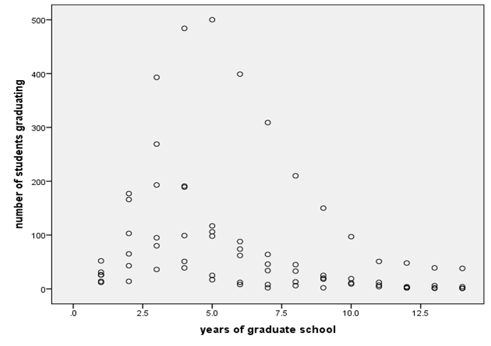
Scatter plot between Year of graduate school and number of students graduating
| Correlations | |||
|---|---|---|---|
| number of students graduating | years of graduate school | ||
| number of students graduating | Pearson Correlation | 1 | -.340** |
| Sig. (2-tailed) | 0.003 | ||
| N | 73 | 73 | |
| years of graduate school | Pearson Correlation | -.340** | 1 |
| Sig. (2-tailed) | 0.003 | ||
| N | 73 | 73 | |
| **. Correlation is significant at the 0.01 level (2-tailed). | |||
Question 2.3
Levene's Test of Equality of Error Variancesa
| F | df1 | df2 | Sig. |
| 14.300 | 5 | 67 | .000 |
| Tests of Between-Subjects Effects | ||||||||||||||||||||||||||||||||||||||||||
|---|---|---|---|---|---|---|---|---|---|---|---|---|---|---|---|---|---|---|---|---|---|---|---|---|---|---|---|---|---|---|---|---|---|---|---|---|---|---|---|---|---|---|
| Dependent Variable: number of students graduating | ||||||||||||||||||||||||||||||||||||||||||
| Source | Type III Sum of Squares | df | Mean Square | F | Sig. | Partial Eta Squared | ||||||||||||||||||||||||||||||||||||
| Corrected Model | 314364.322a | 5 | 62872.864 | 7.298 | 0 | 0.353 | ||||||||||||||||||||||||||||||||||||
| Intercept | 348799.192 | 1 | 348799.192 | 40.484 | 0 | 0.377 | ||||||||||||||||||||||||||||||||||||
| university | 152597.273 | 2 | 76298.636 | 8.856 | 0 | 0.209 | ||||||||||||||||||||||||||||||||||||
| residence | 87246.036 | 1 | 87246.036 | 10.126 | 0.002 | 0.131 | ||||||||||||||||||||||||||||||||||||
| university * residence | 60588.929 | 2 | 30294.465 | 3.516 | 0.035 | 0.095 | ||||||||||||||||||||||||||||||||||||
| Error | 577248.335 | 67 | 8615.647 | |||||||||||||||||||||||||||||||||||||||
| Total | 1336525 | 73 | ||||||||||||||||||||||||||||||||||||||||
| Corrected Total | 891612.658 | 72 | ||||||||||||||||||||||||||||||||||||||||
a. R Squared = .353 (Adjusted R Squared = .304) The univariate Generalized linear model was used to test if the number of student graduating differ among students in different universities and with different residence status. With two main effects identified in this model as university and residence and their interaction term is also included in the model. At a 5% level of significance, the homogeneity assumption is violated in the model from the table above with (F=14.300, p<0.05). Hence, heteroscedasticity is present. The overall model is significant with [F(5,67)=7.298, p<0.05]. This shows there is a significant difference among the number of students graduating from different universities and with different residence statuses. The main effect of the University is significant with [F(2,67)=8.856, p<0.05]. Similarly, the main effect of residence is also significant with [F(1,67)=10.126, p<0.05]. While, the interaction effect is significant too with [F(2,67)=3.516, p<0.05].
Lastly, Eta-Square the effect size measure of this model shows there is a medium effect size across all predictor variables in the model with the least effect size given as 0.095. Question 3.1 A.
| ||||||||||||||||||||||||||||||||||||||||||
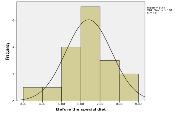
Fig 1: Histogram distribution of before the special diet
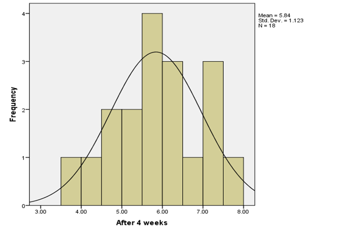
Fig 2: Histogram distribution of diets after 4 weeks
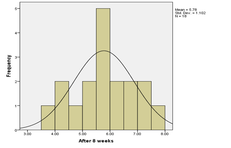
Fig 3: Histogram distribution of diets after 8 weeks
Interpretations

Question 3.2
| Mauchly's Test of Sphericitya | |||||||
|---|---|---|---|---|---|---|---|
| Measure: Cholestrol_levels | |||||||
| Within Subjects Effect | Mauchly's W | Approx. Chi-Square | df | Sig. | Epsilonb | ||
| Greenhouse-Geisser | Huynh-Feldt | Lower-bound | |||||
| Time | 0.381 | 15.44 | 2 | 0 | 0.618 | 0.642 | 0.5 |
| Tests the null hypothesis that the error covariance matrix of the orthonormalized transformed dependent variables is proportional to an identity matrix. | |||||||
| a. Design: Intercept Within Subjects Design: Time |
|||||||
| b. May be used to adjust the degrees of freedom for the averaged tests of significance. Corrected tests are displayed in the Tests of Within-Subjects Effects table. | |||||||
| Tests of Within-Subjects Effects | |||||||
|---|---|---|---|---|---|---|---|
| Measure: Cholestrol_levels | |||||||
| Source | Type III Sum of Squares | df | Mean Square | F | Sig. | Partial Eta Squared | |
| Time | Sphericity Assumed | 4.32 | 2 | 2.16 | 212.321 | 0 | 0.926 |
| Greenhouse-Geisser | 4.32 | 1.235 | 3.497 | 212.321 | 0 | 0.926 | |
| Huynh-Feldt | 4.32 | 1.284 | 3.365 | 212.321 | 0 | 0.926 | |
| Lower-bound | 4.32 | 1 | 4.32 | 212.321 | 0 | 0.926 | |
| Error(Time) | Sphericity Assumed | 0.346 | 34 | 0.01 | |||
| Greenhouse-Geisser | 0.346 | 21.001 | 0.016 | ||||
| Huynh-Feldt | 0.346 | 21.822 | 0.016 | ||||
| Lower-bound | 0.346 | 17 | 0.02 | ||||
| Tests of Between-Subjects Effects | ||||||
|---|---|---|---|---|---|---|
| Measure: Cholestrol_levels Transformed Variable: Average |
||||||
| Source | Type III Sum of Squares | df | Mean Square | F | Sig. | Partial Eta Squared |
| Intercept | 1950.125 | 1 | 1950.125 | 503.326 | 0 | 0.967 |
| Error | 65.866 | 17 | 3.874 | |||
| Estimates | ||||
|---|---|---|---|---|
| Measure: Cholestrol_levels | ||||
| Time | Mean | Std. Error | 95% Confidence Interval | |
| Lower Bound | Upper Bound | |||
| 1 | 6.408 | 0.281 | 5.815 | 7 |
| 2 | 5.842 | 0.265 | 5.283 | 6.4 |
| 3 | 5.779 | 0.26 | 5.231 | 6.327 |
| Pairwise Comparisons | ||||||
|---|---|---|---|---|---|---|
| Measure: Cholestrol_levels | ||||||
| (I) Time | (J) Time | Mean Difference (I-J) | Std. Error | Sig.b | 95% Confidence Interval for Differenceb | |
| Lower Bound | Upper Bound | |||||
| 1 | 2 | .566* | 0.037 | 0 | 0.469 | 0.663 |
| 3 | .629* | 0.042 | 0 | 0.518 | 0.74 | |
| 2 | 1 | -.566* | 0.037 | 0 | -0.663 | -0.469 |
| 3 | .063* | 0.017 | 0.004 | 0.019 | 0.107 | |
| 3 | 1 | -.629* | 0.042 | 0 | -0.74 | -0.518 |
| 2 | -.063* | 0.017 | 0.004 | -0.107 | -0.019 | |
| Based on estimated marginal means | ||||||
| *. The mean difference is significant at the .05 level. | ||||||
| b. Adjustment for multiple comparisons: Sidak. | ||||||