Problem Description:
In a world driven by materialism, the perception of wealth often revolves around outward indicators such as lavish homes, expensive cars, and extravagant lifestyles. This statistical analysis homework aims to challenge this common belief by examining the true characteristics of millionaires. Using data from 274 couples, we delve into the relationship between annual savings and various factors, including education level, combined salary, home and car values, and a "Social Claimer Index." Our goal is to determine whether real millionaires differ from the conventional image of ostentatious wealth, shedding light on the importance of financial prudence and investment.
Solution
Introduction:
The widely acclaimed book, 'The Millionaire Next Door,' questions society's misconception that ostentatious displays of wealth equate to being a millionaire. In truth, genuine millionaires often emerge from unglamorous professions, maintain modest homes and cars, wear budget-friendly attire, and lead unassuming lives while accumulating substantial savings and investments. To test this assertion by Stanley and Danko, we surveyed 274 couples, examining their education level, combined annual salary, home and car values, annual savings, and their self-reported 'Social Claimer Index.' This comprehensive statistical analysis seeks to uncover the true traits of millionaires and their relationship with external symbols of affluence.
Savings:
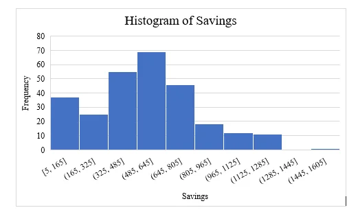
People allocate their income into two categories: savings and consumption. In Figure 1, we present a histogram illustrating the distribution of annual savings among the surveyed couples. This graph reveals that the majority have savings ranging from $485 to $645 per year, with a bell-shaped distribution. However, a closer look shows a segment of couples (approximately 35 to 40) with meager annual savings, falling within the range of $5 to $165. On the opposite side of the spectrum, the chart indicates a dwindling frequency of individuals as savings increase past the peak, signifying that very few couples boast higher savings, with only one couple having between $1445 and $1605 annually.
Figure 1
Histogram of Savings
Relationship of Annual Savings with Education Levels, Combined Salary, Home and Car Values, and the Social Claimer Index:
A correlation matrix (Table 1) provides insights into the connection between annual savings and various factors, including education level, combined salary, home and car values, and the Social Claimer Index. Notably, there is a moderate negative correlation between education level and savings (r = −0.486), the value of homes and savings (r = −0.408), and the Social Claimer Index and savings (r = −0.408). Additionally, a weak negative correlation is observed between combined annual salary and savings (r = −0.162). These findings indicate that increased education, higher earnings, more valuable homes and cars, and greater concern for social status and material possessions correlate with reduced annual savings.
Table 1
Correlation Matrix
| Index | Educ Level | Salary | Cars | Home | Savings | SC Index |
|---|---|---|---|---|---|---|
| Educ Level | 1.000 | |||||
| Salary | 0.382 | 1.000 | ||||
| Cars | -0.105 | 0.542 | 1.000 | |||
| Home | 0.141 | 0.481 | 0.607 | 1.000 | ||
| Savings | -0.486 | -0.162 | -0.381 | -0.408 | 1.000 | |
| SC Index | 0.222 | 0.797 | 0.658 | 0.662 | -0.408 | 1.000 |
Educational Levels & their Respective Annual Savings:
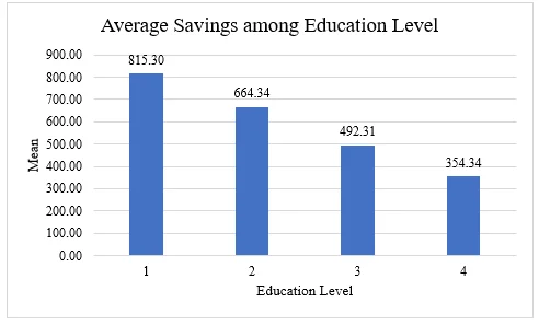
To further explore the influence of education on annual savings, we present a pivot table (Table 2) and a corresponding bar chart (Figure 2). The data reveals that individuals with a high school education only have the highest annual savings, amounting to $815.30, while those with a Doctorate degree exhibit the lowest savings, with an average of $354.34. This implies that higher education is associated with increased expenditures and diminished savings and investments.
Table 2
Mean Savings Among Different Education Levels
| Education Level | Mean Savings ($) |
|---|---|
| High School Only (1) | 815.30 |
| Undergrad Degree (2) | 664.34 |
| Master’s Degree (3) | 492.31 |
| Doctorate (4) | 354.34 |
Figure 2
Bar Chart – Average Savings among Education Level
Combined Annual Salary & Its Effect on Annual Savings:
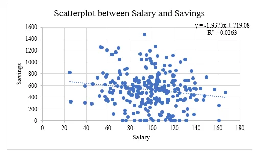
A scatterplot (Figure 3) illustrates the relationship between combined annual salary and annual savings. A clear negative correlation emerges, as the regression line slopes downward. This suggests that as combined annual salary increases, annual savings decrease gradually. However, the low coefficient of determination (R2 = 0.0263) indicates that only 2.63% of the variation in annual savings can be explained by combined annual salary.
Figure 3
Scatterplot between Combined Annual Salary and Annual Savings
Value of Cars & Its Effect on Annual Savings:
Examining the connection between the value of cars and annual savings (Figure 4), we find a notable negative correlation, as the regression line slopes downward. This signifies that as the value of cars increases, annual savings decrease more rapidly. The coefficient of determination (R2 = 0.1461) reveals that 14.61% of the variation in annual savings can be attributed to the value of cars.
Figure 4
Scatterplot between Value of Cars and Annual Savings

Value of Home & Its Effect on Annual Savings:
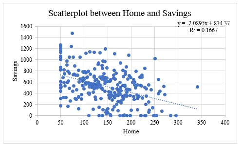
A scatterplot (Figure 5) shows a significant negative relationship between the value of homes and annual savings, with the regression line steeply sloping downward. This indicates that every dollar increase in the value of a home dramatically reduces annual savings. Although the coefficient of determination (R2 = 0.1667) suggests that only 16.67% of the variation in annual savings can be explained by home value, it still outstrips the influence of combined annual salary and the value of cars.
Figure 5
Scatterplot between Value of Home and Annual Savings
Social Claimer Index (SC Index) & Its Effect on Annual Savings:
In Figure 6, we examine the relationship between the Social Claimer Index (SC Index) and annual savings. The regression line illustrates a steep negative correlation, indicating that an increase in the SC Index, reflecting a greater concern for social status and material possessions, substantially reduces annual savings. The coefficient of determination (R2 = 0.1667) suggests that 16.67% of the variation in annual savings is attributed to the SC Index. This demonstrates that the SC Index's impact on annual savings mirrors that of home value, surpassing the influence of combined annual salary and car value.
Figure 6
Scatterplot between Social Claimer Index (SC Index) and Annual Savings
Conclusion:
The study confirms a negative relationship between annual savings and factors such as education level, combined annual salary, home and car values, and the Social Claimer Index. While the strength of these correlations varies, Stanley and Danko's assertion is validated: genuine millionaires often come from unpretentious professions, live modestly, and prioritize savings and investments over extravagant displays of wealth. This research highlights the importance of financial prudence and the need to redefine our perception of true wealth.