Problem Description:
Individuals with clinically significant eating disorders (ED) often experience distorted perceptions of their bodies, which can lead to body image dysmorphia (BID) or body image disturbance. BID is characterized by an individual's obsession with perceived defects in their body, even when these defects are unnoticeable or non-existent. This study aims to investigate how individuals process body size – holistically or in a localized manner. Specifically, it explores whether people tend to focus on specific parts of the body when judging body size. The hypothesis is that when presented with half-body images, individuals will make greater errors in judging body size compared to full-body images. If you need SPSS Assignment Help with this research, feel free to reach out for assistance.
Solution:
Persons with clinically significant eating disorders (ED) such as Anorexia and Bulimia, have distorted conceptions of their bodies. Body image dysmorphia (BID) or Body image disturbance is a person’s preoccupation with the defective body appearance, when the “defects” are unnoticeable or non-existent (Duncam, et al,2016) Many BID sufferers also have atypical visual processing mechanisms (Feusner, Bystritsky, Hellemann, & Bookheimer, 2010
- Data cleaning
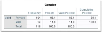
Among the 118 students who provided complete information for this study, 104 representing 88.1% are female while the remaining 14 representing 11.9% are male.
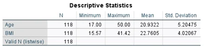
The table above contains summary statistics of both Body Mass Index (BMI) and age. The results show that BMI has a mean of 22.76 with a standard deviation of 4.02 (M = 22.76, SD = 4.02) and age has a mean of 22.93 with a standard deviation of 5.20 (M = 20.93, SD = 5.20). The age of students that participated in this study ranged from 17 to 50 while their ages ranged from 16 to 41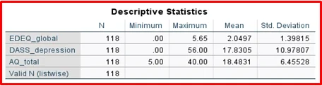
EDEQ global ( M = 2.05, SD = 1.40), DASS depression (M = 17.83, SD = 10.98) and AQ global ( M = 18.48, SD = 6.45). There is more variability in DASS depression than AQ global while EDEQ global has the least variability.
Test of reliability
Internal consistency refers to how well a survey, test, or questionnaire measures to some level of degree what it should actually measure. Cronbach’s alpha is a measure of this reliability.
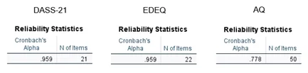
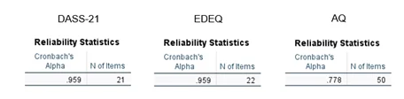
EDE-Q: alpha = .959, DASS-21: alpha = .959 and AQ: alpha = .778
The acceptable value or benchmark for Cronbach’s alpha is between 0.7 and 0.8, between 0.8 and 0.9 is good while 0.9 and above is excellent.
From the reliability statistics presented above, it can be concluded that there is a strong internal consistency or reliability of DASS-21, EDEQ, and AQ. The first two measures (DASS-21 and EDEQ) performed excellently with Cronbach’s alpha 0.959
Inferential stats (testing hypothesis)
– Slopes for 3 conditions e.g., “slope value” (95% CI: lower-upper)
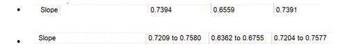
Regression coefficients of the Whole body, top half, and bottom half are presented above. The whole body has a coefficient of 0.7394 with 95% Confidence Intervals of (0.7209, 0.7580) and this implies that we are 95% confident that the true coefficient of the Whole body lies between 0.7209 and 0.7580.
The top half has a coefficient of 0.6559 with 95% Confidence Intervals of (0.6263, 0.6755) and this implies that we are 95% confident that the true coefficient of the top half lies between 0.6263 and 0.6755.
The bottom half has a coefficient of 0.7391 with a 95% Confidence Interval of (0.7204, 0.7577) and this implies that we are 95% confident that the true coefficient of the bottom half lies between 0.7204 and 0.7577.

- R-squared also known as coefficient of determination is a measure of model accuracy. this value measures the percentage of the total variation in the dependent variable explained by the independent variables in the model. R2 for the Whole body is 0.8816 and this means that 88.16% of the total variation in the model is explained by the explanatory variables in the model. Unfortunately, 11.84% could not be explained which is due to random error in the data generating process.
- Similarly, R2 for the top half is 0.8387 and this means that 83.87% of the total variation in the model is explained by the explanatory variables in the model.
- R2 for the bottom half is 0.8803 and this means that 88.03% of the total variation in the model is explained by the explanatory variables in the model.
F-tests to compare 3 conditions e.g., F(DFn, DFd) = “f value”, p = “p-value”
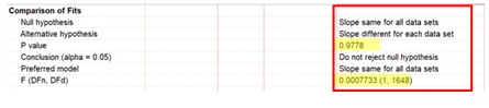
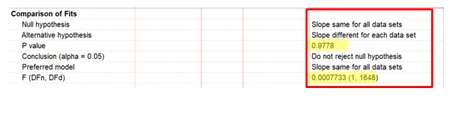
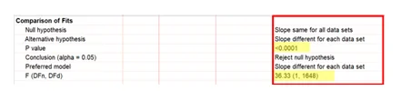
Full body vs bottom half: F(1, 1648) = .0007733, p = .9778, since the p-value (0.9778) is greater than the significance level (0.05), we do not reject the null hypothesis and conclude that all the coefficients are the same for all data set.
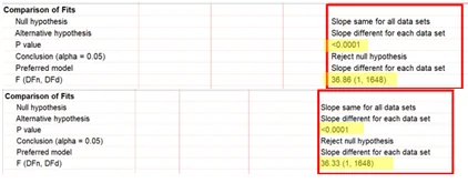
Full body vs top half: F(1, 1648) = 36.86, p = <.0001, since the p-value (0.001) is less than the significance level (0.05), we reject the null hypothesis and conclude that at least one of the slopes is significantly different from others.
Bottom half vs top half: F(1, 1648) = 36.33, p = <.0001, since the p-value (0.001) is less than the significance level (0.05), we reject the null hypothesis and conclude that at least one of the slopes is significantly different from others.
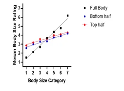
Figure 1. What we expected
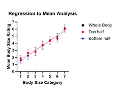
Figure 2. What we saw
Participants
130 first-year and third-year undergraduate psychology students engaged in this study as part of their course. Our sample consisted of 104 females and 14 males, ranging in age from 17 to 50 years. Incomplete data for six participants was removed and, following a performance check removed data of six participants who were unable to discriminate between body size categories resulting in a final Sample, N=118.
Apparatus
Stimuli for this experiment were generated using the CGI program Poser® (2015. ed), the bodyline task, an adaptation of the number line task, was run using Inquisit Player, V:6.6.1 (build: 6581) Model x 86_64 for Windows 10. Microsoft Excel was used to record collected data and SPSS and then Graphpad Prism statistical software to perform analyses. The Eating Disorder Examination (EDE-Q) is the self-reporting questionnaire version of the Eating Disorder There are 28 questions and four subscales. a well-established measurement tool used for both research and clinical purposes to assess eating disorder psychopathology.
and the 21 Question Depression, Anxiety, and Stress Scales (DASS-21) and the Autism Quotient (AQ) were used to characterize our sample group.
AimTo investigate whether individuals process body size holistically or localized manner. (e.g., do they focus on specific parts of the body)
Hypothesis:
Assuming individuals process bodies holistically, it is hypothesized that there will be greater errors in judging the size of the body when presented with the half-body image rather than the full-body image.
Conflicting studies motivate ongoing research into how we estimate body size. Vision studies discovered the phenomena of Serial dependence, a confirmed factor affecting the judgment of body size. Experimenting with inverted body images in contrast to upright presentations, researchers that inversions were no hindrance to judgment, and it seems that the brain is using localized parts of bodies to estimate body estimate size. The results of another study suggest that we perceive size-after-effects, even from resized images and if so, it implies a “holistic” processing for body size. Identifying the neural substrates challenges research design, especially when there are multiple stimuli to consider. It seems likely that because bodies are three-dimensional, our judgment of curves is enhanced for accuracy (Bell, et al., 2013) The integration theory of body size estimation
Design and analysis:
The experiment used a 3 x 7 repeated measures design, with 3 conditions of body size representation and 7 categories of body size. The Bodyline task (Alexi, et al, was presented on ASUS desktop computers with standard 1920 × 1080 screens. MATLAB Data were analyzed using SPSS and GraphPad Prism. The stimuli for this experiment directly reference the Stimuli were 35 real female body images (6.5° × 6.5°), representing seven discrete categories that ranged from extremely thin to extremely large.
A visual noise mask comprised of various pixels from each of the female body images was also implemented. Maintaining a convention for this area of research, and to characterize our sample, we collected trait data using the EDE-Q, the DASS-21, and the AQ questionnaires. Higher scores for trait autism correlate with risk for depression, anxiety, and eating disorders. Analysis of the data from the questionnaires is excluded in this paper due to word count restraints Trait data provides information that may be cross-referenced in extensions of the current paper and related research.
35 CGI body images were generated using Poser CGI software.
One-third of the images were halved to create the top-half and bottom-half body conditions to present for localized visual processing. We matched the appearance of categories 1 & 7 to the real body images in the Alexi et al., 2018 original paper.
Analysis of the data from the bodyline task was entered into Microsoft Excel, and then its regression to the mean was analyzed using SPSS and MATLAB Prism statistical software. A variance to the Alexi design was that we needed to test three times, running the analysis twice more to test data from the top half and bottom half–body conditions.
Procedure
Participants were informed of the nature of the experiment, the tasks to perform, and the protocols in place to protect their identities. After signing informed consent, they completed the bodyline computer task. The task was to position the cursor along the Bodyline, consisting of a line with a range marked from 1.0 to 7.0. The bodyline was anchored at each end by the two extreme body sizes, providing an extended unit of scale beyond the numbered line. During a series of trials, they were presented with a CGI of a female body for 250 ms, followed by a visual noise mask for 500 ms. The visual noise mask was presented to diminish the visual persistence of the image. Participants indicated which body size they saw by clicking the mouse on the bodyline. After completing the bodyline task participants answered a series of questionnaires, the EDE-Q, The DASS-21, and the AQ, and provided details of their weight and height.
– EDE-Q: alpha = .959
– DASS-21: alpha = .959
– AQ: alpha = .778
Descriptive statistics
Participants were 104 females and 14 males, aged between 17 and 50 years (M 20.9322 , SD 5.20475). Participant Body Mass Index (BMI kg/m2 ) ranged from 15.57 to 41.42 (M 22.7605 , SD 4.02067). The participants’ scores on the three questionnaires:
EDE- Q: M = 2.05, SD = 1.40, Range: 0 – 5.65 , DASS depression: M = 17.83, SD = 10.98,
Range: 0 – 56, and for the AQ global: M = 18.48, SD = 6.45, Range: 5 – 40
Table 1
Descriptive Statistics
| Valid |
Female |
104 |
88.1 |
88.1 |
|---|---|---|---|---|
| |
Male |
14 |
11.9 |
100.0 |
| |
Total |
118 |
100.0 |
|
Table 2
Descriptive Statistics
| Age |
118 |
17.00 |
50.00 |
20.9322 |
5.20475 |
|---|---|---|---|---|---|
| BMI |
118 |
15.57 |
41.42 |
22.7605 |
4.02067 |
| Valid N (listwise) |
118 |
|
|
|
|
Cronbach’s alpha was used to check the internal consistency of the DASS-21, the EDEQ-6, and the AQ questionnaires.
Table 3
Results of the Reliability Test for the 3 Questionnaires
| DASS 21 EDE-Q AQ |
|---|
| Reliability Statistics Reliability Statistics Reliability Statistics |
| Cronbach's Cronbach's Cronbach's |
| AIQha N of items AIQha N of items AIQha N of items |
| .959 21. 959 22.778 50 |
Results
Data Cleaning: Participant’s mean body size judgments for each condition was fitted to a linear regression. A slope greater than zero indicated that participants could differentiate between the seven size categories. If a participant rated all seven categories of size as four, then we know they cannot differentiate between sizes, and we removed that data. All statistical analyses were initially recorded in Excel and then run through SPSS Statistics for Windows, with an alpha level of.05, The data was fitted to a linear line before applying an F-test to statistically compare the difference of the slopes. Each of the three conditions was then transposed into a prism for specific comparisons.
There is a slight notable difference between them. but this is proportional to the mean the variance is similar between conditions
To compare the slopes between the three conditions we fitted the data to a linear line and then applied the F-test. The difference between the full-body and half-body conditions and the difference between the two half-body conditions? ( Only the top half of the body image is visible, and only the lower half of the body image is visible)
Bottom half vs top half: F(1, 1648) = 36.33, p = <.0001
Inferential statistics
To test our hypothesis, we
Slopes for 3 conditions e.g., “slope value” (95% CI: lower-upper)
Whole body: .7394 (95% CI: .7209 - .7580)
Top half: .6559 (95% CI: .6362 - .6755)
Bottom half: .7391 (95% CI: .7204 - .7577)
R-squared, is also called the Coefficient of determination The coefficient of determination can be thought of as a percent. It indicates how many data points fall within the results of the line formed by the regression equation; R-square value (goodness of fit) for 3 conditions e.g., R2 = 0.” X”. For the three conditions; Whole body: R2 = .8816, top half: R2 = .8387, and Bottom half: R2 = .8803, all three, expressed as a percent indicate the percentage of points that the line passes through when data points and line are plotted., and for these three conditions, > 80% of the points fall within the regression line, indicating a good fit.
plots the mean size judgment given to each of the seven body categories, on linear axes. The data show that mean body size judgments increase monotonically, and almost linearly with physical body size (R2 = 0.99 for linear fit). This suggests that the size categories were perceived as equidistant. The slope of the linear regression line fitted to the data is less than one, at 0.68 (95% CI: 0.66–0.70).
The distribution for the Coefficient Determination
(R2) for the linear fit. The three conditions are 0.836, and higher suggesting that the categories were judged to be equidistant, and indicated, i.e., clicked on with accuracy. clicked on Regression indexes of the individual subjects 1 minus the slope of best fit linear regression to their bodyline data as an indication of accuracy thresholds, defined as average standard deviations for judgments at each category.
3 x F-tests to compare 3 conditions e.g., F(DFn, DFd) = “f value”, p = “p-value”
Full body vs bottom half: F(1, 1648) = .0007733, p = .9778
For Full body versus top half: F(1, 1648) = 36.86, p = <.0001, we cannot reject the null, the slope is the same for all data sets.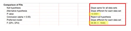
If individuals process bodies holistically, we hypothesized that there would be more errors in body size judgment, when presented with the half-body stimuli than the full-body stimuli.
Greater errors in body size judgments in the top-half condition
However, the body-half condition had an almost identical amount of regression to the mean as the full-body condition
The bottom-half condition shows nearly identical regression to the Mean. This suggests that
Sufficient visual information is present in the bottom half of a body for the brain to accurately estimate the size of the whole body.
Discussion
Our sample was an adequate size to address the question to expect small to medium effect sizes. The Bodyline task is now an established paradigm and is simple for participants. The sufficient difference in the slope for the bottom-half condition is indicative of less error in judgment, a decrease in the number for the top half, indicating more error. The magnitude of error is not different between the whole body and the Bottom half. Our results infer that the bottom- half of a body offers enough visual information, for the brain to construct a size-similar representation for the whole body. Not only does this support our hypothesis, but it is also consistent with the Brooks, et al, 2018 study. Limitations: we acknowledge that the use of CGI or synthetic body images might deprive participants of more natural visual cues because CGI is not 3-dimensional. CGI can represent, but not replicate 3-dimensional curves, visible collarbones, or tissue anomalies.