Tips on how to do linear regression assignment in R with an example
What are some of the basic knowledge in linear regression assignments
The linear regression assignments have common features. The most common identity for linear regression assignment is that any linear regression has two variables: the outcome variable, the dependent variable, and the independent variable. The major assumption for this type of regression is that the relationship between the two variables is linear hence the name. Data analysis can clearly define how the two variables relate to each other. A future dependent variable can also be predicted based on the past outcome.
How to perform explanatory data analysis assignments in R
Before performing the linear regression, R is used to get the background knowledge of the dataset. This is done by plotting the histograms, bar charts and box plots. A frequency distribution table can also be constructed in R for the continuous dataset. The frequency distribution table is a summary statistic indicating the number of observations, standard deviation, median, maximum value, minimum value, range, skewness, kurtosis, and the standard error for each variable. For discrete variables the summary statistics indicate the frequency, percentage, and the cumulative percentage of the variables.
How to interpret the linear regression results from an R output
Linear regression can be observed from an R output in various ways. A scatterplot can be used to show the strength and the direction of the relationship between two or more variables. The contents of the scatterplot can also be presented as a correlation matrix to get the relationship of many variables. An ANOVA table will show the level of significance of the independent variables to the dependent variables. The table will also show the coefficient for each variable
Introduction
Research question: “while controlling for incentives, what is the effect of overtime on workers’ productivity”
The relationship between overtime work and productivity is not direct. While working more can increase the productivity of workers by letting them take advantage of economies of scale, the fatigue that ensue from working for long hours will work the other way around (Gartenstein, 2020). If the opposite effects cancel out each other, over time may have no impact on workers’ productivity (Collewet and Sauermann, 2017). Moreover, when workers are given adequate incentives, they may work for long hours without reducing their productivity. In addition, industrial, firms, and individual specific effect or some external shocks may influence both overtime and productivity which means the effect can be complex than expected. Therefore, it is important to examine the effect of overtime on productivity while factoring the effect of factors mentioned above. The study used data on garment manufacturing industry. The industry is appropriate for this kind of study because garment production is a labour-intensive process. Thus, it is desirable that decision makers in this industry are able to track factors affecting productivity of employees.
Exploratory Data Analysis
The dataset are all control variables. The idle time variable was recoded into a binary variable denoting whether there is idle time or not.
Fig 1 presents the histograms of the continuous variables in the dataset. The histogram is useful in analyzing the distribution of datasets. The plot shows that all the variables are skewed. While prused is the garment manufacturing productivity dataset available atUCI Machine Learning Repository: Productivity Prediction of Garment Employees Data Set. The data consists of 1,197 observations for 15 variables. Important variables for our analysis are productivity which is the dependent variable, overtime which is the main independent variable, number of workers in each team, number of style changes for a particular product, allocated time for a task, incentives and idle time which oductivity is left skewed; overtime, time allocated for tasks, incentives and number of workers are skewed to the right. The skewness is more pronounced and extreme for incentives.
The box plots of the variables are presented in fig 2. The boxplot is useful to check the distribution of the variables as well as the presence or otherwise of outliers. The outlier values of dataset are labeled outside the plot. As observed from the plot, minutes of overtime worked have one outlier value while productivity and incentives have several outlier values.
Fig 3 presents the bar chart of the two categorical variables in the dataset: number of style change for a particular product and idle time. The plot shows that style did not change for 1,050 observation and this constitutes 87.7% of dataset as shown in fig 4. 114 of production constituting 9.5% have style change once while 33 (2.8%) of production have style changed twice. There was no idle time in 1179 of the production which means 98.5% of the production is without idle time. on the other hand, idle time was observed in 1.5% (18) of the production.
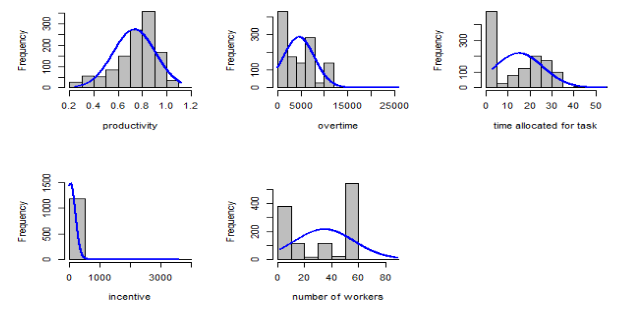
Fig : Histogram
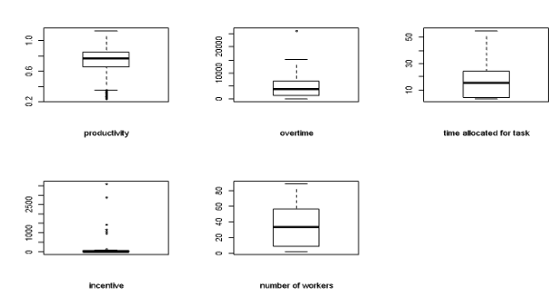
Fig 2: Box plot of Continuous Variables
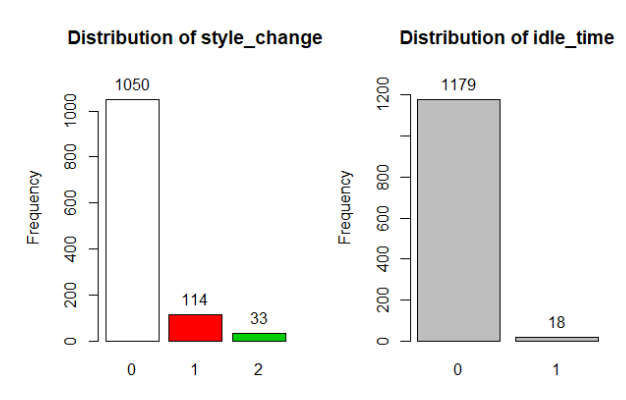
Fig 3: Bar Chart of Style Change and Idle Time
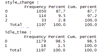
Fig 4: Frequency Distribution of style of change and idle time
Figure 5 presents the summary statistics of the continuous variables in the dataset, the result shows that average productivity is 0.74 while the variation around the mean is given by the standard deviation of 0.17. Since, there are outliers in the dataset, it is more appropriate to summarize by the median. The median value is 0.77. Productivity ranges from 0.23 to 1.12. Median overtime minutes is 3960 minutes and ranges from 0 minutes to 3960 minutes. Median value for incentives is 0 while the mean is 38.21. this wide difference between mean and median demonstrate how vulnerable the mean value is to outliers. The highest incentive given is 3600. The skewness and kurtosis value is very large which demonstrates huge departure from normality. Average number of time allocated for task (smv) is 15.06 minutes while the median is 15.26 minutes. The lowest minutes allocated is 2.9 minutes while the highest minutes allocated is 54.56 minutes. Average number of workers in each team is approximately 35 people while the median is 34 people. The team with the least number of people have 2 members while the team with the highest number of people has 89 members.
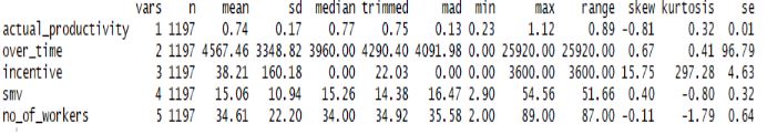
Fig 5: Summary Statistics
The scatter plot and correlation matrix is presented in figure 7 and 6 respectively. The result shows there is negative, insignificant correlation between overtime and productivity at 5% level of significance (r=-0.05, p=0.06). Weak, positive and significant correlation was found between productivity and incentive (r=0.077, p=0.008). Negative and weak but significant correlation was found between productivity and time allocated (r=-0.12, p<.001), no of style changes (r=-0.21, p<.001), no of workers (r=-0.06, p=0.04) and idle time (r=-0.17, p<.001). Between the independent variables, there is a very strong and positive correlation between number of workers and time allocated for task (r=0.9). Similarly strong correlation was found between overtime and number of workers (r=0.73) and between overtime and number of minutes allocated (r=0.67).
The scatter plot shows the relationships graphically. It is observed that some relationships are influenced by outliers in the dependent or independent variables and may actually impact the regression results. The correlation and scatterplot suggests that there is probably no significant effect of overtime on productivity while reverse is the case for incentives.
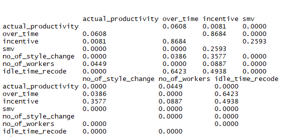
Fig 6: Correlation
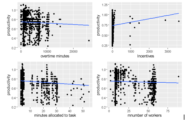
Figure 7: Scatterplot
Linear Regression
Question set I
From the scatter plot in figure 7, we observed that a fairly linear relationship exists between productivity and overtime minutes, minutes allocated to task and probably incentives because the points on the plot do not form a pattern that suggests non normality. Conversely, a linear relationship does not exist between number of workers and productivity as the points on the pattern shows a polynomial of order three.
The correlation presented in figure 6 shows that there are a number of significantly correlated variables among the independent variables. For example, number of workers and time allocated for task, overtime and number of workers, overtime and number of minutes allocated. The correlation between number of workers and time allocated for task is worrisome because the correlation is greater than 0.9 which may be a source of multicollinearity. To guard against this, we remove one of the variables
The regression result is summarized in figure 8. The result shows that parameters for incentive, idle time and number of style change are significant while overtime minutes and time allocated are not significant. The main independent variable (over time) is not significantly correlated with productivity and has no significant effect after controlling for other variables. However, it has significant correlations with three of the five control variables. Minutes allocated on the other hand is significantly correlated with the dependent variable and is correlated with the main predictor and all other control variables except incentives. Idle time is significantly correlated with the dependent variable but not the main predictor and incentive.
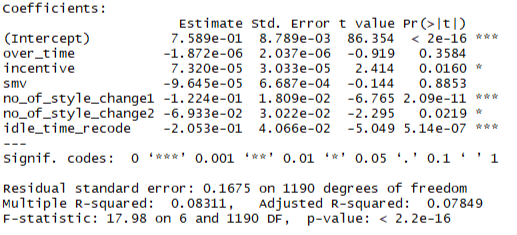
Figure 8: Regression Result
Since one of the two insignificant predictors is the main predictor, we cannot remove it, we only remove the control variable that is not significant. The result is presented in fig 9. We see that the estimated parameters for other predictors increased a bit when we remove one insignificant parameter. The coefficient of the intercept however reduced a bit.
The p-value of the parameters of the predictors reduced when we remove the insignificant parameters except for incentive which slightly increased from 0.0160 to 0.0161. A look at the correlation shows that both variables are not significantly correlated which may be the reason for the non-response of its p-value parameter to the removal.
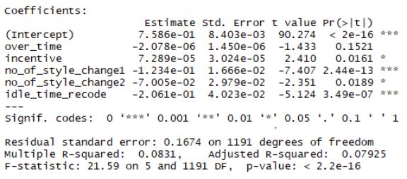
Figure 9: Regression Result
The 95% alt="Confidence interval
"confidence interval is presented in fig 10. For a significant parameter, zero must not fall within this interval. We see from the result that only overtime and time allocated have zero within their interval which means they are not significant. A parameter which have zero between its 95% confidence interval will have its p-value greater than 0.05 as observed for overtime and time allocated.
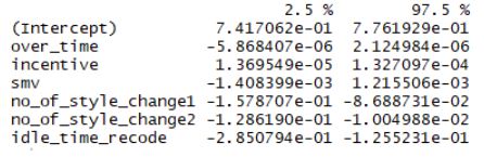
figure :10 Regression Result
The R2 is the percent of variation in dependent variable that is explained by the independent variables in the model. The R2 from our model is 0.0831 which means that the independent variables accounts for 8.31% of variation in the productivity.
Question Set II
The regression model where all variables are significant is selected by a stepwise removal of non-significant variables from the initial model. The result shows we have only three explanatory variables which are incentive, idle time and no of style change. The parameter of this model can be interpreted as the effect of the respective predictor on productivity while holding other predictors constant.
The interpretation of estimated signs depends on the type of variable. for continuous variable like incentive, the positive sign means that a thousand BDT increase in incentive will increase productivity by 0.07. However, for factor variables like no of style change and idle time, the estimates is the difference in average value of one level compared to the base level. For example, the coefficient of number of style change 1 indicates that average productivity is lower when the style is changed once than when it is not changed at all by 0.12. Similarly, the coefficient of number of style change 2 indicates that average productivity is lower when the style is changed twice than when it is not changed at all by 0.07. Moreover, average productivity is lower by 0.2 when there is idle time compared to when there is no idle time.
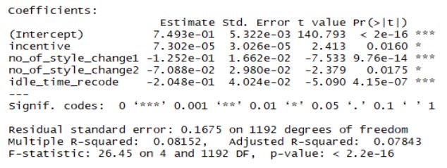
Figure 11: Regression Result
For a unit change in one of the predictors, idle time have the largest influence on the predictor variable.
Given that we have variables that are treated as categorical, to predict for a new case we need to make assumption about the value they take as their average will not make sense. Based on this, we assume that there is no style change (no_of_style_change=0) and there is no idle time (idle_time_recode=0). The prediction and confidence interval is presented below
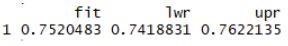
Fig 12: prediction for new case at mean of predictors
The result shows that the average productivity at average incentives and when there is no style change and there is no idle time is 0.75 with the 95% confidence interval between 0.74 and 0.76
Similarly, the result at the 90th percentile of incentives under the same assumption for idle time and no of style change is shown in fig 13.
Figure 13: prediction for new case at 90% percentiles of predictors
The result shows that the average productivity at 90% percentile of incentives and when there is no style change and there is no idle time is 0.7 with the 95% confidence interval between 0.74 and 0.76. We observed that productivity is high when we use 90th percentile than when productivity is average
Conclusion
The study sets out to answer whether overtime have significant effect on productivity after controlling for incentives. Descriptive statistics, correlation and regression were used for the study. The graphical analysis shows that all variables are skewed and there are considerable outliers in some of the variables. No significant correlation was found between productivity and overtime but significant correlation was found between incentives and productivity. The multiple regression result shows that even after controlling for incentives and other variables, there is no significant effect of overtime on productivity but incentives significantly affect productivity. We conclude that there working overtime does not impact the productivity of garment industry workers but incentives do. The insignificant effect may be due to positive and negative effect of overtime canceling out one another or that the incentives is high such that it canceled out the fatigue associated with working overtime.
Given more time, I would have performed diagnostic test to determine the validity of the model in terms of meeting assumptions of classical linear regression. This is necessary to give credence to the result. Moreover, I will add more variables and determine their relevance so that the model can include all relevant variables and all information possible is captured. This will increase model fits and ensure more accurate prediction can be made.
References
Collewet, M., & Sauermann, J. (2017). Working hours and productivity. Labour Economics, 47, 96–106. doi:10.1016/j.labeco.2017.03.006
Gartenstein, D (2020). Relationship between overtime & productivity. Work - Chron.com. https://work.c mhron.com /relationship-between-overtime-productivity-2952.html
R code
productivity=read.csv("garments_worker_productivity.csv")
head(productivity)
View(productivity)
library(rcompanion)
par(mfrow=c(2,3))
plotNormalHistogram(productivity$actual_productivity,xlab="productivity")
plotNormalHistogram(productivity$over_time,xlab="overtime")
plotNormalHistogram(productivity$smv,xlab="time allocated for task")
plotNormalHistogram(productivity$incentive,xlab="incentive")
plotNormalHistogram(productivity$no_of_workers,xlab="number of workers")
par(mfrow=c(2,3))
boxplot(productivity$actual_productivity,xlab="productivity")
boxplot(productivity$over_time,xlab="overtime")
boxplot(productivity$smv,xlab="time allocated for task")
boxplot(productivity$incentive,xlab="incentive")
boxplot(productivity$no_of_workers,xlab="number of workers")
productivity$idle_time_recode=ifelse(productivity$idle_time==0,0,1)
library(epiDisplay)
par(mfrow=c(1,2))
style_change=productivity$no_of_style_change
idle_time=productivity$idle_time_recode
tab1(style_change)
tab1(idle_time)
library(psych)
cont=productivity[,c(15,9,10,7,14)]
describe(cont)
library(PerformanceAnalytics)
cor_data=productivity[,c(15,9,10,7,13,14,16)]
chart.Correlation(cor_data,histogram =F,pch=19)
library(ggplot2)
g1=ggplot(cor_data,aes(x=over_time,y=actual_productivity))+
geom_point()+
geom_smooth(formula = y~x)+
labs(x="overtime minutes",y="productivity")
g2=ggplot(cor_data,aes(x=incentive,y=actual_productivity))+
geom_point()+
geom_smooth(formula = y~x)+
labs(x="Incentives",y="productivity")
g3=ggplot(cor_data,aes(x=smv,y=actual_productivity))+
geom_point()+
geom_smooth(formula = y~x)+
labs(x="minutes allocated to task",y="productivity")
g4=ggplot(cor_data,aes(x=no_of_workers,y=actual_productivity))+
geom_point()+
geom_smooth(formula = y~x)+
labs(x="mnumber of workers",y="productivity")
library(gridExtra)
grid.arrange(g1,g2,g3,g4,ncol=2,nrow=2)
##regression
cor_data$no_of_style_change=factor(cor_data$no_of_style_change)
mod=lm(actual_productivity~.,data=cor_data)
summary(mod)
c2=cor_data[,-6]
modb=lm(actual_productivity~.,data=c2)
summary(modb)
c3=c2[,-4]
modc=lm(actual_productivity~.,data=c3)
summary(modc)
confint(modb)
c4=c3[,-2]
modd=lm(actual_productivity~.,data=c4)
summary(modd)
newdata=data.frame(incentive=mean(productivity$incentive),no_of_style_change=0,idle_time_recode=0)
newdata$no_of_style_change=factor(newdata$no_of_style_change)
pred=predict(modd,newdata,se.fit=T,interval="confidence",level=0.95)
pred$fit
newdata2=data.frame(incentive=quantile(productivity$incentive,prob=0.9),no_of_style_change=0,idle_time_recode=0)
newdata2$no_of_style_change=factor(newdata2$no_of_style_change)
pred2=predict(modd,newdata2,se.fit=T,interval="confidence",level=0.95)
pred2$fit