Estimating Regression Model and Performing Hypothesis Test Using STATA
Regression modeling and hypothesis testing are two of the most intricate concepts every stat student should know. Regression modeling involves developing a function that explains the relationship between one or multiple independent variables and a target variable, also known as a dependent or response variable. On the other hand, a hypothesis test is all about making an educated guess. Researchers use it to test if a survey or experiment results are meaningful. Both hypothesis testing and regression modeling can be done using STATA. Students facing hurdles with projects based on hypothesis tests and regression modeling usually avail of our STATA assignment help. To prove to you that we are equal to the task, we have prepared a solution for STATA homework that requires us to estimate regression models by given equations using STATA. We have also specified the econometric model and analyzed the empirical findings based on the econometric estimation and the hypothesis test. Our statistics homework help service can be accessed anytime by students who need assistance with similar assignments.
Model and Theoretical Foundation
The model of consumption expenditures is a relationship between consumption expenditure and income. The model was first formulated by Keynes who propose that consumption increase with income but less than proportionately i.e. as income increases by 1%, consumption also increases but by less than 1% which means that the marginal propensity to consume is zero. The income which consumption depends on have been given different interpretation by economist. According to Keynes's absolute income hypothesis, the income is the current income of the consumer which means that consumer only considers their current income when making consumption decision. However, theorists after Keynes recognize the fact that consumer considers their lifetime resources when making consumption decisions. Milton Friedman proposes the permanent income hypothesis which posits that consumers make consumption decisions based on their permanent income but not transitory income. On the other hand, Modigliani and Brumberg (1954) and Ando and 8 Modigliani (1963) propose the life-cycle hypothesis which argued that consumers smoothen consumption over their lifetime.
Econometric Model
The simple consumption model can be specified in an econometric model as shown below:
C=β_1+β_2 Y+u_i
Where C represents consumption, and Y represents income, u represents the error term. The β_1 and β_2 are parameters that represent the autonomous consumption and marginal propensity to consume respectively. Both are expected to be greater than 0. In addition, β_2 is expected to be less than 1.
The model can be modified to include control variables such as
C=β_1+β_2 Y+β_3 cshpi+β_4 csent+u_i
Where cshpi represents the US home price index while csent is the consumer sentiment index.
Consumption is usually affected during a recession because income is reduced and purchasing power is reduced. The model can thus be modified to include the effect of recession.
C=β_1+β_2 Y+β_3 cshpi+β_4 csent+β_5 increc+u_i
Where increase is the interaction of Y and a dummy variable which equals 1 when there is recession and 0 otherwise.
Data Source and Variables
The data is collected from the database of the Federal Reserve Bank of St Louis. The variables and their description is shown in table 1.
Table 1: Description of Variables
| Variable | Description | Unit of measurement |
| C | US real personal consumption expenditures | Billions of chained 2012 dollars |
| Y | US real disposable personal income | Billions of chained 2012 dollars |
| cshpi | Seasonally adjusted S&P/Case-Shiller US Home Price Index | Index (Base year=2000:M1) |
| cshpi | University of Michigan Consumer Sentiment Index | Index (Base year=1996:Q1) |
| rec | Dummy variable represents if the US is in recession | 1 if the U.S. economy was in a recession
0 otherwise |
d. Result
The estimated result of the three models is presented in table 2. Panel 1 presents the result of the simple model. The result showed that there is a positive and significant effect of income on consumption. The MPC is 0.694 which means that if income increases by $1, consumption increases by $0.69. The autonomous consumption (intercept) is $2517.98 which means that consumers spent $2517.98 on consumption when they have no income.
For the second model, after controlling for the house price index and consumer sentiment, the MPC is 0.595 which means that if income increases by $1, consumption increases by $0.6. The autonomous consumption is $2315.13 which means that consumers spent $2315.13 on consumption when they have no income. Both the house price index and consumer sentiment have a positive and significant effect on consumption. If the house price index increases by $1, consumption increases by $5.95 while if the consumer sentiment index increase by one unit, consumption increases by $5.1.
For the third model, after including the interaction of recession and disposable income, the coefficient of this interaction is negative and significant which means MPC is greater when there is no recession that when there is a recession. The MPC when there is no recession is 0.59 while the MPC when there is a recession is 0.59-0.02=0.57. This implies that if income increases by $1, consumption increases by $0.59 when there is no recession and $0.57 when there is a recession.
Table 2: Estimated Result
Model (1) | Model (2)
| Model (3) | |
| dispincome | 0.694***
(0.015) | 0.595***
(0.024) | 0.590***
(0.024) |
| cshpi | 5.951***
(1.257) | 6.228***
(1.246) | |
| csent | 5.096*
(2.143) | 2.082
(2.403) | |
| increc | -0.021**
(0.008) | ||
| _cons | 2517.976***
(189.009) | 2315.128***
(245.182) | 2598.471***
(264.771) |
| N
R2 F p>F | 241.000
0.9005 2172.956 <.001 | 241.000
0.9118 827.945 <.001 | 241.000
0.9140 638.422 <.001 |
Standard errors in parentheses
*p< 0.05, **p< 0.01, ***p< 0.001
The R2 for these models ranges from 0.901 to 0.914 which means that the independent variables account for between 90.1% and 91.4% of the variation in personal consumption. The F-stat for all the models is significant (p<.001) which means that the independent variables are jointly significant.
Diagnostic Test for Model 3
The model is tested for autocorrelation, heteroscedasticity, omitted variable bias, multicollinearity, and normality. The result is presented in Table 3
The autocorrelation test showed that the null hypothesis of no autocorrelation is rejected (χ^2=135.12,p<.001) which implies that the model suffers from autocorrelation. The heteroscedasticity test showed that the null hypothesis of no heteroscedasticity is rejected (χ^2=270.03,p<.001) which implies that the model suffers from heteroscedasticity. The Ramsey RESET test for omitted variable bias showed that the null hypothesis of no omitted variable is rejected (F=113.81,p<.001) which implies that the model suffers from omitted variable bias.
Table 3: Diagnostic test result
| Test | Statistics(p) |
| Breusch-Godfrey LM test for autocorrelation | 135.12(<.001) |
| heteroscedasticity | 270.03 (<.001) |
| Omitted variable test | 113.81 (<.001) |
The variance inflation factor test is used to test for multicollinearity. The result presents evidence of no multicollinearity as none of the variables have VIF greater than 10.
| Variable | VIF | 1/VIF |
| chspi | 3.12 | 0.320870 |
| dispincome | 3.04 | 0.328254 |
| csent | 1.34 | 0.744450 |
| increc | 1.29 | 0.772662 |
| Mean VIF | 2.20 |
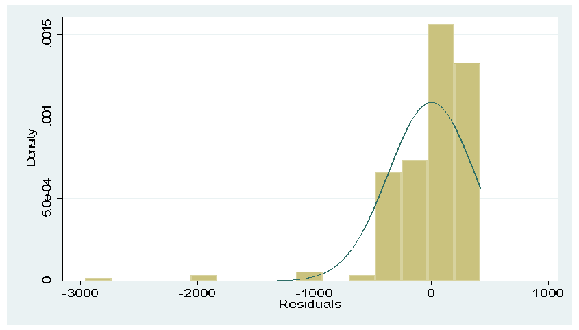
The histogram below is used to test for the normality of the residuals. The plot showed that the histogram of residuals is skewed to the left which means that the normality assumption is violated.
 f. Analysis and Suggestions
The results support the proposition of economists regarding the relationship between income and consumption. In all variations of the models, income has a significant impact on consumption. In addition, the economic theory proposition regarding the direction and magnitude of the marginal propensity to consume and autonomous consumption was supported by the result. However, the model suffers a violation of major assumptions of classical linear regression like autocorrelation, multicollinearity, omitted variable bias, and normality of residuals. Therefore, this casts doubt on the correctness of the model. Thus, the model should be modified by first including the lags of consumption as it is theoretically sensible that present consumption will depend on past consumption because consumers will try to maintain past consumption levels even in the face of falling income. This will correct the autocorrelation problem if the lag is correctly specified and may partially or fully correct the omitted variable bias. Also, the robust standard error can be used to take care of heteroscedasticity