Creating and Exploring SPSS Data
A. Create an SPSS data set using the following information. Include screenshots of the data view, variable view and any procedures used.
1. In addition to inputting the data, make sure you format the columns in variable view if appropriate.
2. Binary categorical variables should be coded as dummy variables.
3. All variables except Student name should be numeric
| Student | Jimmy | Peter | Erica | Jessica | Melissa | Joe | Mark | Carrie | Maggie | Jeremy | Claudia | Susan | Paul |
|---|---|---|---|---|---|---|---|---|---|---|---|---|---|
| Marital Status | single | married | divorced | divorced | single | single | married | single | single | married | single | married | single |
| Study:hours studied for exam | 2 | 10 | 0 | 4 | 7 | 15 | 4 | 11 | 3 | 30 | 6 | 6 | 9 |
| University | UTEP | NMSU | UTEP | UTEP | NMSU | NMSU | NMSU | UTEP | NMSU | NMSU | NMSU | UTEP | NMSU |
| Exam: Percent | 73 | 82 | 70 | 94 | 90 | 88 | 78 | 82 | 80 | 98 | 94 | 85 | 92 |
| Exam: Grade | C | B | C | A | A | B | C | B | B | A | A | B | A |
| Anexiety Score: Scale of 1-10 | 9 | 7 | 5 | 4 | 3 | 5 | 2 | 8 | 4 | 5 | 6 | 4 | 4 |
B. Perform the following on your newly created dataset (calculate=by hand/calculator, not using SPSS; illustrate your work)
1. Calculate and interpret the mean for the University dummy variable.
Mean = 1106/13 = 85.07692
2. For the exam Percent variable
a. calculate and interpret the mean, median and mode
Mean = 85.07692%
The Median is the 7th number when the numbers are arranged in ascending order. The median is equal to 85
Mode of the distribution is equal to 82, as it is the most common number
b. calculate the Standard Deviation
Standard deviation = 8.536
c. Calculate the 95% confidence interval for the mean (note small sample size)
95% confidence interval = (71.934, 99.436)
d. Calculate the z-scores for Melissa, Joe and Jeremy.
Z-score for Melissa = 0.726
Z-score for Joe = 0.534
Z-score for Jeremy = 2.046
e. What is the probability that someone would score as high or higher than Melissa? What is the probability that someone would score in between Joe and Jeremy? (Hint: where do you go to find z-score probabilities?)
P (Score higher than Melissa) = 0.43
P (Score between Joe and Jeremy) = 0.622
Checking for Mean, Standard Deviations, Confidence Interval and Z-scores
3. Now check your calculations for the variable Exam by having SPSS provide you with the mean, standard deviations, 95% confidence interval and z-scores. Copy and paste any SPSS table as part of your answer and explain how you produced the results in SPSS.
| Statistics | ||
| Exam_percent | ||
| N | Valid | 13 |
| Missing | 0 | |
| Mean | 85.0769 | |
| Median | 85.0000 | |
| Mode | 82.00a | |
| Std. Deviation | 8.53875 | |
| Skewness | -.265 | |
| Std. Error of Skewness | .616 | |
| Minimum | 70.00 | |
| Maximum | 98.00 | |
| a. Multiple modes exist. The smallest value is shown | ||
Comparing Two Variables
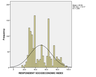
C. Compare the two variables Tvhours (Hours of TV per day) and Sei (Socioeconomic Index).
1. Which of the two variables has a higher amount of variability. Explain how you reached your conclusion (hint: you need to account for the difference in the unit of measurement by using an equation explained in the lecture notes).
| Descriptive Statistics | |||||||
| N | Minimum | Maximum | Mean | Std. Deviation | Skewness | ||
| Statistic | Statistic | Statistic | Statistic | Statistic | Statistic | Std. Error | |
| HOURS PER DAY WATCHING TV | 987 | 0 | 24 | 3.02 | 2.675 | 2.993 | .078 |
| RESPONDENT SOCIOECONOMIC INDEX | 1360 | 17.1 | 97.2 | 49.843 | 19.1702 | .464 | .066 |
| Valid N (listwise) | 926 | ||||||

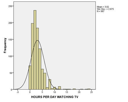
D. Chart a frequency distribution (Histogram) for the tv hours watched (tvhours) and describe the distribution.

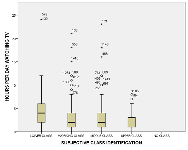
E. Createboxplots of respondents hours of tv watched (tvhours)by social class (class). You should have one graph with 4 side by side boxplots, one for each social class. Use the graphs to answer the following questions.

1. Which social class has the highest median hours of tv watching? Estimate this median from the graph.
2. Which social class has the highest interquartile range of tv watching? Estimate this interquartile range from the graph.
3. Describe the shape of the distribution of tv watching for the upper class.
Check your answers by obtaining the actual numbers using an SPSS procedure. Provide the results, including a screenshot of the output.
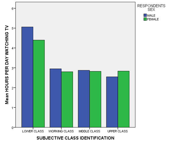
F. Explore the comparison further by examining how tv watching (tvhours) varies by both social class (class) and gender (sex). Create one bar chart which takes into consideration both gender and socioeconomic status. Based on the graph, explain the patterns in the data.

Running Analyses and Interpreting
Please continue to use the same dataset for questions 1-3. Provide information on how you completed the steps by including a description of the steps you took in constructing the analysis and screenshots.
Below you are given a series of research problems. Use the appropriate statistical technique to test the hypotheses. You will use a different SPSS procedure for each of the questions. The procedures we covered for this exam are One-Sample T-Test, Independent Sample T-Test, and Crosstabs. You will use each of the 3 types of analysis at least once, however, so you might want to go through the exam first to determine which procedure you are going to use on which question. Make sure you thoroughly discuss the output and not just leave it up to my interpretation. Here are some guidelines for what you should cover in your answers. Make sure you revisit these for each question so you don’t forget what to include in your answer.
For all 3 research problems, you will need to
- Identify the IV and DV and the level of measurement for each. Assume a critical alpha of p<.05 for all 3 analyses.
- Identify which of the 3 statistical techniques you are using and explain why?
- State the null and research hypotheses (in words).
- Complete the analysis using the appropriate SPSS procedure. Provide screenshots of procedure and output.
- Make sure to identify the test statistic value and corresponding p-value.
- Discuss whether the result is significant and whether you reject or fail to reject the null hypothesis. If significant, identify the probability that you just committed a type 1 error.
- Interpret the output by providing a statement about the relationship or lack of relationship between the variables and the direction of the result, if appropriate.
- If confidence intervals are given in the output, provide a statement interpreting the confidence interval.
In addition, for each specific technique, you will need to
Independent Sample T-Test
• Assess the homogeneity of variance assumption (i.e. equal variances assumption) using the Levene’s test.
Crosstab with Chi-Square
• Check for significance across columns and within cell residuals.
• Provide and interpret at least one measure of association.
1. Two of your friends are arguing about whether married people are happier than non-married people. One friend believes that getting married makes people happier and the other one believes that once you are married life is a drag. You agree to settle their argument by examining the GSS dataset from your statistics class. Conduct your analysis with the variables “marital” and “happy”.
| GENERAL HAPPINESS * MARITAL STATUS Crosstabulation | |||||||
| Count | |||||||
| MARITAL STATUS | Total | ||||||
| MARRIED | WIDOWED | DIVORCED | SEPARATED | NEVER MARRIED | |||
| GENERAL HAPPINESS | VERY HAPPY | 265 | 25 | 48 | 5 | 62 | 405 |
| PRETTY HAPPY | 367 | 74 | 134 | 20 | 222 | 817 | |
| NOT TOO HAPPY | 54 | 27 | 48 | 18 | 77 | 224 | |
| Total | 686 | 126 | 230 | 43 | 361 | 1446 | |
| Chi-Square Tests | |||
| Value | df | Asymptotic Significance (2-sided) | |
| Pearson Chi-Square | 117.866a | 8 | .000 |
| Likelihood Ratio | 117.256 | 8 | .000 |
| Linear-by-Linear Association | 82.414 | 1 | .000 |
| N of Valid Cases | 1446 | ||
| a. 0 cells (0.0%) have expected count less than 5. The minimum expected count is 6.66. | |||
After explaining your results, you realize that this relationship might not be the same for men and women. Test to see if there is a conditional relationship. Explain your results.
2. One important area of study for sociologists is stratification, which includes patterns of inequality. One common way to operationalize inequality in sociology is socioeconomic status (in the GSS sei is an index constructed from a combination of questions regarding the individual’s occupation, education and income). Let’s use the GSS data to analyze patterns of income inequality.
Gender has historically been a strong predictor of inequality. Test the research hypothesis that women’s socioeconomic status (sei) is lower on average than men’s.
| Group Statistics | |||||||||||||||
| RESPONDENTS SEX | N | Mean | Std. Deviation | Std. Error Mean | |||||||||||
| RESPONDENT SOCIOECONOMIC INDEX | MALE | 597 | 51.270 | 19.9521 | .8166 | ||||||||||
| FEMALE | 763 | 48.726 | 18.4719 | .6687 | |||||||||||
| Independent Samples Test | |||||||||||||||
| Levene's Test for Equality of Variances | t-test for Equality of Means | ||||||||||||||
| F | Sig. | t | df | Sig. (2-tailed) | Mean Difference | Std. Error Difference | 95% CI of the Difference | ||||||||
| Lower | Upper | ||||||||||||||
| RESPONDENT SOCIOECONOMIC INDEX | Equal variances assumed | 4.542 | .033 | 2.434 | 1358 | .015 | 2.5447 | 1.0h456 | .4935 | 4.5958 | |||||
| Equal variances not assumed | 2.411 | 1230.576 | .016 | 2.5447 | 1.0555 | .4740 | 4.6154 | ||||||||
3. The average age of the U.S. population is 37.7 years old. Test to see whether our sample is younger or older than the U.S. population.
| One-Sample Statistics | ||||
| N | Mean | Std. Deviation | Std. Error Mean | |
| AGE OF RESPONDENT | 1433 | 49.21 | 17.563 | .464 |
| One-Sample Test | ||||||
| Test Value = 37.7 | ||||||
| t | df | Sig. (2-tailed) | Mean Difference | 95% Confidence Interval of the Difference | ||
| Lower | Upper | |||||
| AGE OF RESPONDENT | 24.818 | 1432 | .000 | 11.514 | 10.60 | 12.42 |