Part 1 - Subscription Dataset Analysis
Problem Description:
This take-home assessment focuses on analyzing two datasets, Subscription.csv, and Amusement.csv, using the R programming language. It assesses your ability to examine data, perform data transformations, conduct exploratory data analysis, and draw meaningful insights. Below is a breakdown of the homework's key components:
Solution
Q1. Please examine the nature of the dataset. In your examination, make sure that you list (10 pts)
(i) the number of rows (respondents) and number of columns (variables), (ii) the data types of each variable, (iii) the first 15 rows of the dataset, (iv) whether there is any missing value in the dataset, (v) some of the variables are character types, convert them into factors because we will need them in the factor type for analysis. After you convert the character to a factor type variable, make sure that it is converted (with an R function), (vi) run summary statistics of the dataset.
i. There are 298 rows and 7 columns
> subscription=read.csv("subscription.csv")
> dim(subscription)
[1] 298 7
ii. the data types of each variable
> str(subscription)
'data. frame': 298 obs. of 7 variables:
$ age: num 23.3 25.9 24.7 61.3 24.2 ...
$ gender: chr "Male" "Female" "Female" "Female" ...
$ income: num 11985 12406 12545 15347 15493 ...
$ kids: int 1 0 1 0 1 0 0 3 2 0 ...
$ ownHome: chr "ownNo" "ownNo" "ownNo" "ownYes" ...
$ subscribe: chr "subNo" "subNo" "subYes" "subNo" ...
$ Segment: chr "Urban hip" "Urban hip" "Urban hip" "Travelers" ...
iii. the first 15 rows of the dataset
head(subscription,15)
age gender income kids own home subscribe Segment
- 23.25671 Male 11985.25 1 ownNo subNo Urban hip
- 25.94617 Female 12406.10 0 ownNo subNo Urban hip
- 24.69923 Female 12544.68 1 ownNo subYes Urban hip
- 61.32715 Female 15346.68 0 ownYes subNo Travelers
- 24.24272 Male 15493.40 1 ownNo subNo Urban hip
- 22.75965 Female 15910.54 0 ownNo subYes Urban hip
- 22.34075 Male 16341.09 0 ownNo subNo Urban hip
- 21.36267 Male 16646.48 3 ownNo subNo Urban hip
- 21.49348 Female 17082.74 2 ownNo subNo Urban hip
- 25.93903 Female 17366.86 0 ownNo subNo Urban hip
- 23.33063 Male 17382.01 4 ownNo subNo Urban hip
- 23.19013 Male 17510.28 1 ownNo subYes Urban hip
- 25.15129 Male 17757.67 1 ownNo subNo Urban hip
- 23.49583 Male 17784.57 1 ownNo subNo Urban hip
- 23.97756 Male 18106.84 0 ownNo subNo Urban hip
iv. whether there is any missing value in the dataset
> sum(is.na(subscription))
[1] 0
v. Converting character type to factor type
> gender=as.factor(subscription$gender)
> ownHome=as.factor(subscription$ownHome)
> subscribe=as.factor(subscription$subscribe)
> Segment=as.factor(subscription$Segment)
>
> str(gender)
Factor w/ 2 levels "Female","Male": 2 1 1 1 2 1 2 2 1 1 ...
> str(ownHome)
Factor w/ 2 levels "ownNo","ownYes": 1 1 1 2 1 1 1 1 1 1 ...
> str(subscribe)
Factor w/ 2 levels "subNo","subYes": 1 1 2 1 1 2 1 1 1 1 ...
> str(Segment)
Factor w/ 4 levels "Moving up","Suburb mix",..: 4 4 4 3 4 4 4 4 4 4 ...
vi. summary statistics of the dataset
> library(dplyr)
> subscription=mutate_if(subscription,is.character,as.factor)
> str(subscription)
'data. frame': 298 obs. of 7 variables:
$ age: num 23.3 25.9 24.7 61.3 24.2 ...
$ gender: Factor w/ 2 levels "Female","Male": 2 1 1 1 2 1 2 2 1 1 ...
$ income: num 11985 12406 12545 15347 15493 ...
$ kids: int 1 0 1 0 1 0 0 3 2 0 ...
$ ownHome: Factor w/ 2 levels "ownNo","ownYes": 1 1 1 2 1 1 1 1 1 1 ...
$ subscribe Factor w/ 2 levels "subNo","subYes": 1 1 2 1 1 2 1 1 1 1 ...
$ Segment: Factor w/ 4 levels "Moving up","Suburb mix",..: 4 4 4 3 4 4 4 4 4 4 ...
> summary(subscription)
summary(subscription)
age gender income kids' ownhome
Min. :19.26 Female:157 Min. : 11985 Min. :0.000 ownNo :159
1st Qu.:32.97 Male :141 1st Qu.: 39966 1st Qu.:0.000 ownYes:139
Median:39.43 Median: 52200 Median:1.000
Mean:41.12 Mean: 51298 Mean:1.279
3rd Qu.:47.85 3rd Qu.: 61437 3rd Qu.:2.000
Max. :80.49 Max. :114278 Max. :7.000
subscribe Segment
subNo:258 Moving up: 70
subYes: 40 Suburb mix:100
Travelers: 78
Urban hip: 50
Q2. The dataset has a variable called “subscribe” (whether the person is subscribed to a service or not). Please sort the data based on subscription behavior (subNo vs subYes) and come up with the Summary statistics for each subscription behavior separately. For each set, please discuss age, gender, income, number of kids, whether they own a home or not, and what customer segment they belong to. Based on the output do you see any difference between people who subscribe to the service and who don't subscribe to the service? (10 pts)
> newdata=subscription[order(subscribe),]
> summary(newdata[newdata$subscribe=="subYes", ])
age gender income kids townhome
Min. :21.24 Female:21 Min. :12545 Min. :0.00 ownNo :22
1st Qu.:29.69 Male :19 1st Qu.:35155 1st Qu.:0.00 ownYes:18
Median:36.57 Median:49107 Median:1.00
Mean:39.65 Mean:45934 Mean:1.25
3rd Qu.:47.02 3rd Qu.:56145 3rd Qu.:2.00
Max. :80.49 Max. :82077 Max. :6.00
subscribe Segment
subNo : 0 Moving up:14
subYes:40 Suburb mix: 6
Travelers:10
Urban hip:10
> summary(newdata[newdata$subscribe=="sub no", ])
age gender income kids ownHome
Min. :19.26 Female:136 Min. : 11985 Min. :0.000 ownNo :137
1st Qu.:33.16 Male :122 1st Qu.: 40637 1st Qu.:0.000 ownYes:121
Median:39.78 Median: 52883 Median:1.000
Mean:41.35 Mean: 52130 Mean:1.283
3rd Qu.:47.85 3rd Qu.: 62830 3rd Qu.:2.000
Max. :78.20 Max. :114278 Max. :7.000
subscribe Segment
subNo:258 Moving up:56
subYes: 0 Suburb mix:94
Travelers:68
Urban hip:40
Discussion: out of 288 people, only 40 subscribed while the remaining 258 did not subscribe. Among the 40 people that subscribed, 21 are female while 19 are male. 18 own a home while 22 do not own a home. 14 of them are moving up segment, 16 are in the Suburb mix while 10 are in both Travelers and Urban. Among the 258 people who do not subscribe, 136 are female while 122 are male. 121 own a home while 137 do not own a home. 56 of them are in the moving up segment, 94 are in the Suburb mix, 68 are in Travelers and 40 are in Urban.
The average age of people who subscribe is 39.65 while the mean age of people who do not subscribe is 41.35; the average income of people who subscribe is 45,934while the average income of people who do not subscribe is 52,130, the highest number of kids owned by those that subscribe is 6 while 7 kids is the maximum for the those that do not subscribe.
Q3. There are two subscription statuses: Yes or No. Please create cross-tables and a proportion-based cross-table between subscription status and (i) home ownership, (ii) gender, (iii) segments. And please briefly interpret the overall findings at the end (10 pts)
> table(subscription$subscribe, subscription$gender)
Female Male
subNo 136 122
subYes 21 19
> table(subscription$subscribe, subscription$Segment)
Moving up Suburb mix Travelers Urban hip
subNo 56 94 68 40
subYes 14 6 10 10
>
> prop.table(table(subscription$subscribe, subscription$ownHome))
ownNo ownYes
subNo 0.45973154 0.40604027
subYes 0.07382550 0.06040268
> prop.table (table(subscription$subscribe, subscription$gender))
Female Male
subNo 0.45637584 0.40939597
subYes 0.07046980 0.06375839
> prop.table(table(subscription$subscribe, subscription$Segment))
Moving up Suburb mix Travelers Urban hip
subNo 0.18791946 0.31543624 0.22818792 0.13422819
subYes 0.04697987 0.02013423 0.03355705 0.03355705
The result show that 46% of people that do not subscribe are female while 41% are male, also, only 7% of those that subscribe are female while the remaining subscribers representing just 6% are male.
Among the four segments, 18.8% do not subscribe while 4.7% actually subscribed in the Moving up segment. 31.5% do not subscribe while 2.0% subscribed in the Suburb segment. 22.8% do not subscribe while 3.4% subscribed in the Travelers segment. Finally, 13.4% do not subscribe while 3.5% subscribed in the Urban hip segment.
Q4. Let’s examine the data even further to understand the segments. Please find out what the average income, average number of kids, and average age is for each segment. Please interpret the findings briefly (15 pts)
> aggregate(subscription$income,list(subscription$Segment),FUN=mean)
Group.1 x
- Moving up 53090.97
- Suburb mix 55033.82
- Travelers 63884.52
- Urban hip 21681.93
> aggregate(subscription$kids,list(subscription$Segment),FUN=mean)
Group.1 x
- Moving up 1.914286
- Suburb mix 1.920000
- Travelers 0.000000
- Urban hip 1.100000
> aggregate(subscription$age,list(subscription$Segment),FUN=mean)
Group.1 x
- Moving up 36.33114
- Suburb mix 39.92815
- Travelers 57.98783
- Urban hip 23.88459
Among the four segments, on average we have an income of 53,090.97, an average age of 36.3, and an average of 2 kids in the Moving up segment. We have an average income of 55,033.82, an average age of 39.9, and an average of 2 kids in the Suburb mix segment. We have an average income of 63,884.52, an average age of 58, and an average of 0 kids in the Travelers segment; finally, We have an average income of 63,884.52, an average age of 23.9 and an average of 1 kid in the Urban hip segment.
This means that the Travelers segment has the highest income and age but with the lowest number of kids. People in Urban Hip have the lowest income and age with a kid on average.
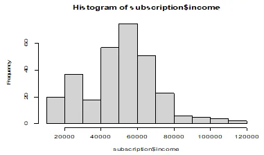
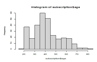
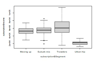
Q5. Please create a (i) a histogram for income and discuss it distribution, (ii) a histogram for age and discuss its distribution, (iii) a boxplot for income vs. customer segments (note: income is on the x-axis, customer segments are on the y-axis) and (iv) a boxplot for age vs. customer segments (note: age is on the x-axis, customer segments are on the y-axis). Please interpret the findings in brief (20 pts).
hist(subscription$income)
hist(subscription$age)
boxplot(subscription$income~subscription$Segment)
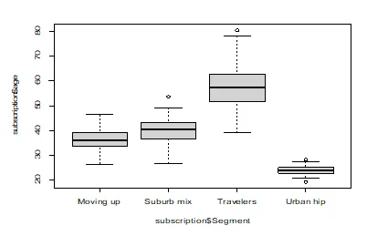
boxplot(subscription$age~subscription$Segment)
Both income and age displayed on the histogram above deviate considerably from normal distribution. This is due to the non-symmetrical shape of their histograms. In particular, both income and age are positively skewed to the right.
The histogram of age and income across segments shows that there is a difference between Travelers and Urban hubs in income and age. However, both the Suburb mix and Moving segments tend to have the same income and age.
Q6. Please find out (i) the mean income for each segment, (ii) the mean age for each segment, (iii) the mean number of kids for each segment, (iv) the total number of homeownerships for each segment, (v) total number of subscription for each segment, (vi) the total number of males and females in each segment. Please interpret the findings (20 pts).
> aggregate(subscription$income,list(subscription$Segment),FUN=mean)
Group.1 x
- Moving up 53090.97
- Suburb mix 55033.82
- Travelers 63884.52
- Urban hip 21681.93
> aggregate(subscription$kids,list(subscription$Segment),FUN=mean)
Group.1 x
- Moving up 1.914286
- Suburb mix 1.920000
- Travelers 0.000000
- Urban hip 1.100000
> aggregate(subscription$age,list(subscription$Segment),FUN=mean)
Group.1 x
- Moving up 36.33114
- Suburb mix 39.92815
- Travelers 57.98783
- Urban hip 23.88459
> table(subscription$ownHome,subscription$Segment)
Moving up Suburb mix Travelers Urban hip
ownNo 47 52 20 40
ownYes 23 48 58 10
> table(subscription$subscribe,subscription$Segment)
Moving up Suburb mix Travelers Urban hip
subNo 56 94 68 40
subYes 14 6 10 10
> table(subscription$gender,subscription$Segment)
Moving up Suburb mix Travelers Urban hip
Female 49 48 40 20
Male 21 52 38 30
In the Moving Up segment, there are 23 people who own a home while 47 do not own a home, 14 people subscribe while 56 people do not subscribe, and 49 people are females while 21 are males.
In the Suburb mix segment, there are 48 people who own a home while 52 do not own a home, 6 people subscribe while 94 people do not subscribe, and 48 people are females while 52 are males.
In the Travelers segment, there are 58 people who own a home while 20 do not own a home, 10 people subscribed while 68 people do not subscribe, and 40 people are females while 38 are males.
In the Urban hip segment, there are 10 people who own a home while 40 do not own a home, 10 people subscribe while 40 people do not subscribe, and 20 people are females while 30 are males.
Q7. When you bring the results together, what do you recommend the company to do so that they can increase the number of their subscription service customers? (20 pts.)
Out of the 298 people, only 40 representing 13.42% subscribed. There are differences between people who have subscriptions and who do not have subscriptions to craft strategies. 121 people own a home and do not subscribe to craft strategies; Even though the income and age distribution are not normal, the company should try as much as possible to reach out to a larger percentage of non-subscribers as this will help in increasing the number of people who subscribe to craft strategies.
Part 2 - Amusement Dataset Analysis
Problem Description: The Amusement.csv dataset contains responses from visitors to an amusement park, detailing their satisfaction levels with various aspects of their experience, along with additional variables.
Solution
Q8. Please examine the nature of the dataset. In your examination, make sure that you list: (i) the number of rows (respondents) and number of columns (variables), (ii) the data types of each variable, (iii) whether there is any missing value in the dataset, (iv) run summary statistics of the dataset. (10 pts)
> amusement=read.csv("amusement.csv")
> dim(amusement)
[1] 500 8
> str(amusement)
'data. frame': 500 obs. of 8 variables:
$ weekend: chr "yes" "yes" "no" "yes" ...
$ num. child: int 0 2 1 0 4 5 1 0 0 3 ...
$ distance: num 114.6 27 63.3 25.9 54.7 ...
$ rides: int 87 87 85 88 84 81 77 82 90 88 ...
$ games: int 73 78 80 72 87 79 73 70 88 86 ...
$ wait: int 60 76 70 66 74 48 58 70 79 55 ...
$ clean: int 89 87 88 89 87 79 85 83 95 88 ...
$ overall: int 47 65 61 37 68 27 40 30 58 36 ...
> sum(is.na(amusement))
[1] 0
> summary(amusement)
weekend num. child distance rides
Length:500 Min. :0.000 Min. : 0.5267 Min. : 72.00
Class :character 1st Qu.:0.000 1st Qu.: 10.3181 1st Qu.: 82.00
Mode: character Median:2.000 Median: 19.0191 Median: 86.00
Mean:1.738 Mean: 31.0475 Mean: 85.85
3rd Qu.:3.000 3rd Qu.: 39.5821 3rd Qu.: 90.00
Max. :5.000 Max. :239.1921 Max. :100.00
games wait clean overall
Min. : 57.00 Min. : 40.0 Min. : 74.0 Min. : 6.00
1st Qu.: 73.00 1st Qu.: 62.0 1st Qu.: 84.0 1st Qu.: 40.00
Median: 78.00 Median: 70.0 Median: 88.0 Median: 50.00
Mean: 78.67 Mean: 69.9 Mean: 87.9 Mean: 51.26
3rd Qu.: 85.00 3rd Qu.: 77.0 3rd Qu.: 91.0 3rd Qu.: 62.00
Max. :100.00 Max. :100.0 Max. :100.0 Max. :100.00
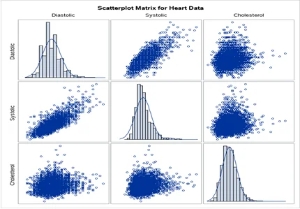
Q9. Run a scatterplot matrix for all the variables in the data (note: first access the “car” library to be able to run the scatterplot matrix). Check the distribution of each variable. List the ones that are normally distributed and non-normally distributed. Transform the ones that are not normally distributed [note: please use log() transformation is now. you can use any transformation method you want. Make sure that the variable is normally distributed after the transformation, provide evidence that they are normally distributed after the transformation](20 pts)
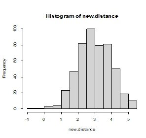
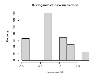
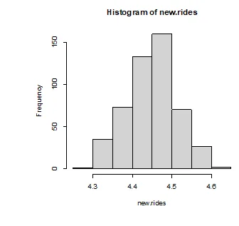
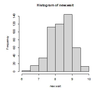
The variables that are normally distributed are overall, clean, and games. The variables that are not normally distributed are number of children, distance, rides, and wait. After applying logarithmic and square transformations on the non-normal variables, they all show signs of normality as displayed below.
library(car)
scatterplot matrix(~amusement$num.child+amusement$distance+amusement$rides+amusement$games+amusement$wait+amusement$clean+amusement$overall)
> new.distance=log(amusement$distance)
> new.num.child=log(amusement$num.child)
> new.rides=log(amusement$rides)
> new.wait=sqrt(amusement$wait)
>hist(new.distance)
> hist(new.num.child)
> hist(new.rides)
> hist(new.wait)
Q10. Run the plot for the variables: “overall” satisfaction and “rides” satisfaction. Add a regression line to evaluate the strength of the relationship between these variables (note: you are not running a regression analysis, instead just add a regression line to evaluate the direction and strength of the relationship). Please discuss the findings. (15 pts)
plot(amusement$rides,amusement$overall)
> abline(lm(amusement$overall~amusement$rides),col="red")
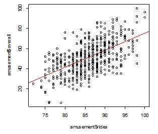
The plot suggests a positive linear relationship between overall satisfaction and ride satisfaction. This means that an increase in overall satisfaction is associated with ride satisfaction and vice versa.
BONUS (10 pts). Please provide your opinion on the course, its content, and its execution. [your bonus points will be proportional to the volume of insight you provide]
- Do you face any challenges and struggles in learning R and if yes, which aspect(s) do you find most challenging in your learning experience?
- So far, thinking about what we have learned in the class with R, what aspects of R do you like?
- What aspects of the course do you find positive about your learning experience?
- What aspects of the course can be improved to contribute to your learning experience? [basically, what else can be done/or differently done to enhance your learning process]